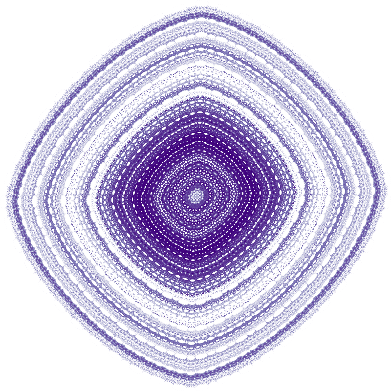
Plotting Hopalong attractor with Datashader and Numba
What is an attractor? Definition from wikipedia:
In the mathematical field of dynamical systems, an attractor is a set of numerical values toward which a system tends to evolve, for a wide variety of starting conditions of the system. System values that get close enough to the attractor values remain close even if slightly disturbed. An attractor is called strange if it has a fractal structure.
Most of the following code comes from James Bednar’s notebook about 2D strange attractor plotting with Datashader, which was inspired by an entry from Lazaro Alonso, I think.
Datashader is a great Python library that allows to create beautiful images from large amout of spatial data, e.g. census data. Numba is an open-source NumPy-aware optimizing compiler for Python, used here to quickly compute the trajectories.
Here I focus on Hopalong attractor, introduced by Barry Martin. You can see the definition here (hopalong_1). I also found another slight different definition here (hopalong_2) along with some sets of parameter values. Some other parameter values were taken from here. Finally, I stumbled on this nice (but rather hypnotic) webgl Hopalong Orbits Visualizer.
import numpy as np
import pandas as pd
import datashader as ds
from datashader import transfer_functions as tf
import numba
from numba import jit
import matplotlib
import matplotlib.pyplot as plt
import warnings
warnings.filterwarnings("ignore")
import sys

print(f"Python version: {sys.version}")
print(f"Numpy version: {np.__version__}")
print(f"Pandas version: {pd.__version__}")
print(f"Datashader version: {ds.__version__}")
print(f"Matplotlib version: {matplotlib.__version__}")
Python version: 3.7.0 (default, Jun 28 2018, 13:15:42)
[GCC 7.2.0]
Numpy version: 1.15.1
Pandas version: 0.23.4
Datashader version: 0.6.6
Matplotlib version: 2.2.3
# image size
width = 800
height = 800

# number of steps
n = 10000000

# colormap
purples = plt.get_cmap('Purples')
Martin map functions
These 2D maps have three fixed parameters: a, b and c. For a given set of (x, y) values, it returns a new one. This corresponds to a single iteration.
@jit
def hopalong_1(x, y, a, b, c):
    return y - np.sqrt(np.fabs(b * x - c)) * np.sign(x), \
           a - x

@jit
def hopalong_2(x, y, a, b, c):
    return y - 1.0 - np.sqrt(np.fabs(b * x - 1.0 - c)) * np.sign(x - 1.0), \
           a - x - 1.0
Trajectory function
We take x, y = 0, 0 as initial condition and then apply a Martin map n-1 times.
@jit
def trajectory(fn, a, b, c, x0=0, y0=0, n=n):
    x, y = np.zeros(n), np.zeros(n)
    x[0], y[0] = x0, y0
    for i in np.arange(n-1):
        x[i+1], y[i+1] = fn(x[i], y[i], a, b, c)
    return pd.DataFrame(dict(x=x,y=y))
Visualization function
The trajectory function returns a dataframe with x and y coordinates (a vector of n points). Next we aggregate these points into a 2D grid in order to count the number of points per grid cell, which is in turn transfomed into a color.
cvs = ds.Canvas(plot_width=width, plot_height=height)

def compute_and_plot(fn, a, b, c):
    df = trajectory(fn, a, b, c)
    agg = cvs.points(df, 'x', 'y')
    return tf.Images(tf.shade(agg, cmap=purples))
Resulting images
%%time
compute_and_plot(hopalong_1, 2.0, 1.0, 0.0)
CPU times: user 1.62 s, sys: 149 ms, total: 1.77 s
Wall time: 1.06 s
%%time
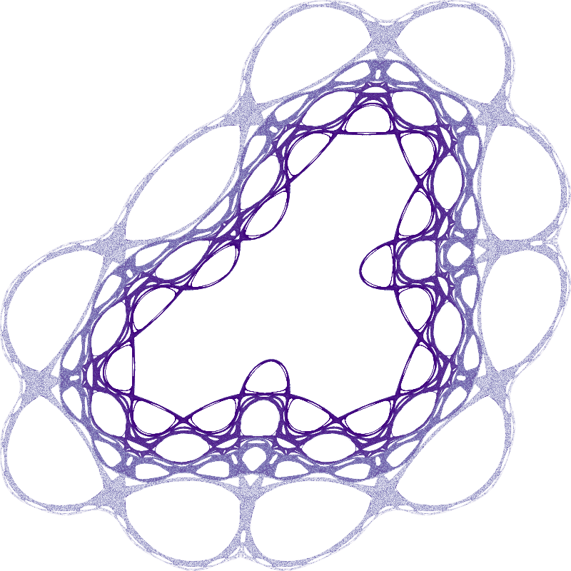
compute_and_plot(hopalong_1, -11.0, 0.05, 0.5)
CPU times: user 721 ms, sys: 161 ms, total: 882 ms
Wall time: 379 ms

%%time
compute_and_plot(hopalong_1, 2.0, 0.05, 2.0)
CPU times: user 861 ms, sys: 167 ms, total: 1.03 s
Wall time: 434 ms
%%time
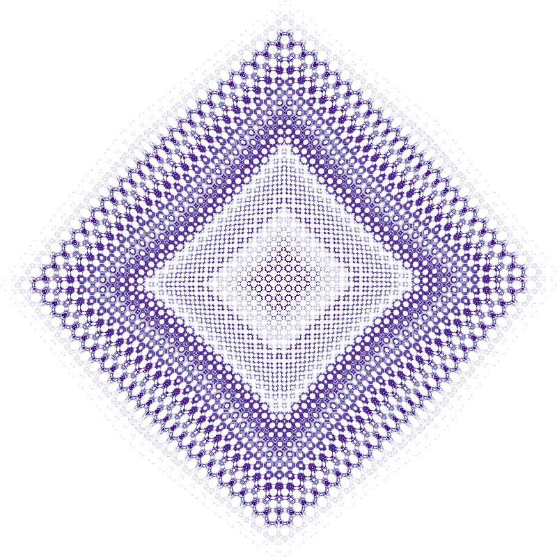
compute_and_plot(hopalong_1, 0.1, 0.1, 20.0)
CPU times: user 678 ms, sys: 164 ms, total: 842 ms
Wall time: 364 ms
%%time
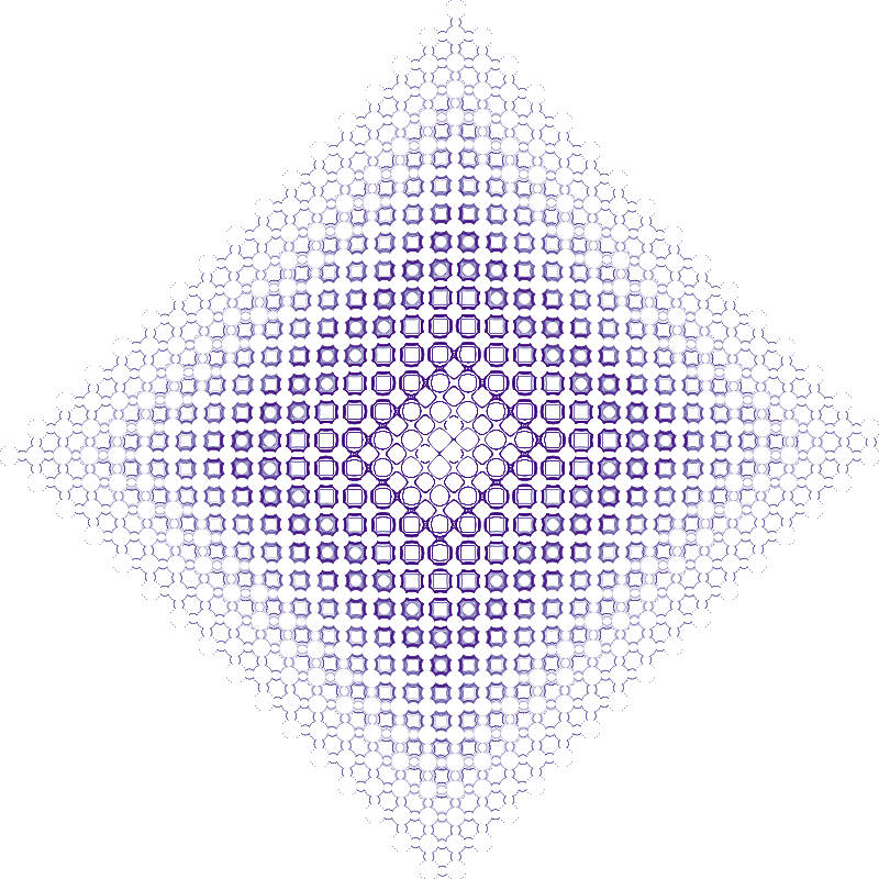
compute_and_plot(hopalong_1, 1.1, 0.5, 1.0)
CPU times: user 782 ms, sys: 132 ms, total: 914 ms
Wall time: 381 ms
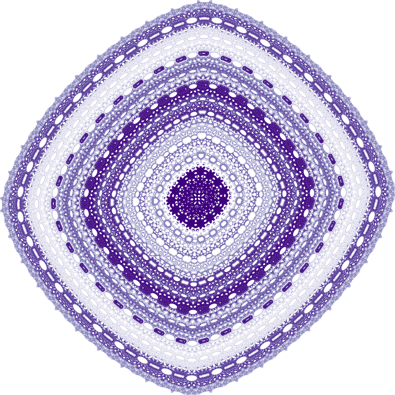
%%time
compute_and_plot(hopalong_2, 7.16878197155893, 8.43659746693447, 2.55983412731439)
CPU times: user 884 ms, sys: 140 ms, total: 1.02 s
Wall time: 620 ms
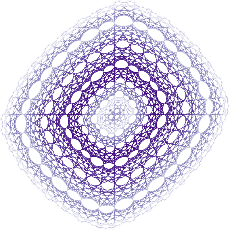
%%time
compute_and_plot(hopalong_2, 7.7867514709942, 0.132189802825451, 8.14610984409228)
CPU times: user 756 ms, sys: 299 ms, total: 1.05 s
Wall time: 470 ms
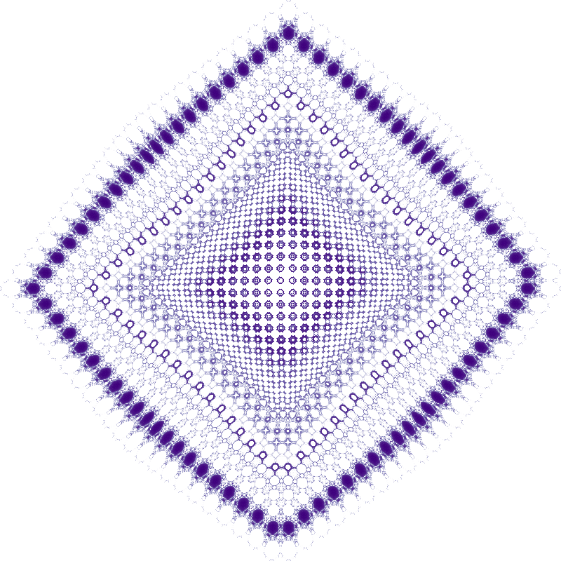
%%time
compute_and_plot(hopalong_2, 9.74546888144687, 1.56320227775723, 7.86818214459345)
CPU times: user 703 ms, sys: 152 ms, total: 855 ms
Wall time: 378 ms
