Loading data into a Pandas DataFrame - a performance study

Because doing machine learning implies trying many options and algorithms with different parameters, from data cleaning to model validation, the Python programmers will often load a full dataset into a Pandas dataframe, without actually modifying the stored data. This loading part might seem relatively long sometimes… In this post, we look at different options regarding the storage, in terms of elapsed time and disk space.
We are going to measure the loading time of a small- to medium-size table stored in different formats, either in a file (CSV file, Feather, Parquet or HDF5) or in a database (Microsoft SQL Server). For the file storage formats (as opposed to DB storage, even if DB stores data in files…), we also look at file size on disk.
Measurements are going to be performed for different tables lengths, table widths and “data entropy” (number of unique values per columns).
This performance study is inspired by this great post Extreme IO performance with parallel Apache Parquet in Python by Wes McKinney.
Introduction
Let’s start by giving the complete list of the storage formats evaluated in the present post, describing the hardware and software environment, as well as the fake data set.
Complete list of storage formats
Here is the list of the different options we used for saving the data and the Pandas function used to load:
- MSSQL_pymssql : Pandas’ read_sql() with MS SQL and a pymssql connection
- MSSQL_pyodbc : Pandas’ read_sql() with MS SQL and a pyodbc connection
- MSSQL_turbobdc : Pandas’ read_sql() with MS SQL and a turbobdc connection
- CSV : Pandas’ read_csv() for comma-separated values files
- Parquet_fastparquet : Pandas’ read_parquet() with the fastparquet engine. File saved without compression
- Parquet_fastparquet_gzip : Pandas’ read_parquet() with the fastparquet engine. File saved with gzip compression
- Parquet_pyarrow : Pandas’ read_parquet() with the pyarrow engine. File saved without compression
- Parquet_pyarrow_gzip : Pandas’ read_parquet() with the pyarrow engine. File saved with gzip compression
- Feather : Pandas’ read_feather()
- HDF_table : Pandas’ read_hdf(). File saved with the
tableoption. From Pandas’ documentation:write as a PyTables Table structure which may perform worse but allow more flexible operations like searching / selecting subsets of the data
- HDF_fixed : Pandas’ read_hdf(). File saved with the
fixedoption. From Pandas’ documentation:fast writing/reading. Not-appendable, nor searchable
Data creation
For the purpose of the comparison, we are going to create a fake table dataset of variable length n, and variable number of columns:
n_intcolumns ofint64type, generated randomnly in the between 0 andi_max-1,n_floatcolumns offloat64type, drawn randomly between 0 and 1,n_strcolumns ofcategorytype, of categorigal data withn_catuniquestrin each column (n_catdifferent words drawn randomly from Shakespeare’s King Lear)
So we have a total of n_col = n_int + n_float + n_str columns. The parameters i_max and n_cat control the “level of entropy” in the integer and categorical columns, i.e. the number of unique values per column.
df = create_table(n=2, n_int=5, n_float=5, n_str=5, i_max=50, n_cat=10, rng=rng)
print(df)
   I00  I01  I02  I03  I04       F00       F01       F02       F03       F04  \
0   18   27   46    9   17  0.394370  0.731073  0.161069  0.600699  0.865864
1    3   11   26   28   11  0.983522  0.079366  0.428347  0.204543  0.450636

        S00   S01       S02        S03     S04
0      Cure  deer  unsettle    weakens  wicked
1  banished  wrap     Loyal  fortnight  wicked
Hardware
All measurements are performed on the same laptop with these feats:
- CPU: Intel(R) Core(TM) i7-7700HQ (8 cores) @2.80GHz
- RAM: DDR4-2400, 16GB
- Disk: Samsung SSD 970 PRO NVMe M.2, 1TB (average read rate: 3,3 GB/s)
Libraries
We use the Anaconda distibution of CPython 3.7.3and the following package versions:
| package | version |
|---|---|
| pandas | 0.24.2 |
| sqlalchemy | 1.3.5 |
| pymssql | 2.1.4 |
| pyodbc | 4.0.24 |
| turbodbc | 3.1.1 |
| fastparquet | 0.3.1 |
| pyarrow | 0.13.0 |
| tables | 3.5.2 |
Time measurements and equality tests
When measuring the reading time, we always keep the best out of three successive measurements.
Note that only the HDF_table format support writing and reading columns of category type. So for all the other formats, categorical columns are converted back into dtype=category after being read (this operation is included in the reading time measurement). Actually,
we also make sure that the list of the different categories is always in lexicographical order:
categories = CategoricalDtype(list(df[col].unique()), ordered=True)
df[col] = df[col].astype(categories)
For the HDF_fixed format, one further have to explicitly convert the categorical column into strings before writing the dataframe into a file.
Also, we checked that the read data is exactly the same as the written data by using a small dataframe (only a few rows), storing it in each format, reading it and comparing the input and output dataframes:
pd.testing.assert_frame_equal(df_written, df_read)
Results
First, we change the table length but keep a fixed number of columns, then vary the number of columns with a fixed length. Finally we are going to change the number of unique values in each int and category columns (for a fixed number of rows and columns).
Loop on different lengths
We loop on different table lengths n, from 10 to 1000000, with the following set of parameter values: n_int=5, n_float=5, n_str=5, i_max=50, n_cat=10.
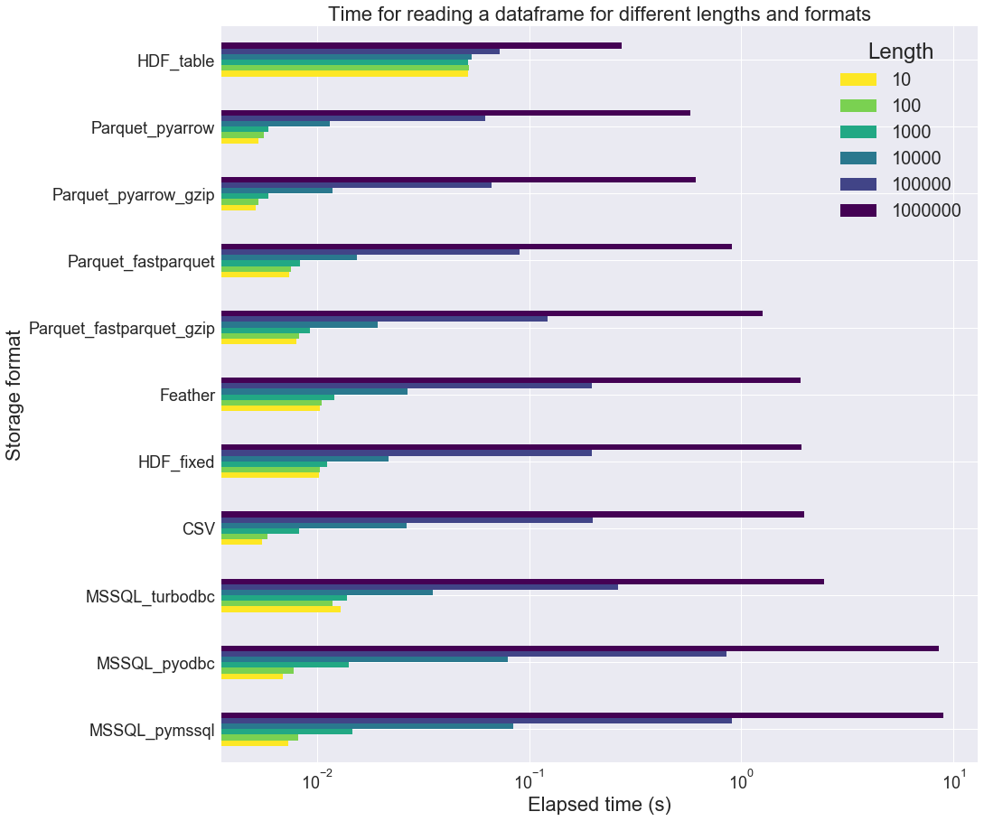
In the above figure, the format are sorted in ascending order of reading time for the largest table length (n=1000000). This is why the HDF_table format appears first. However we can observe that this format performs poorly on small table sizes. Overall, Parquet_pyarrow is the fastest reading format for the given tables. The Parquet_pyarrow format is about 3 times as fast as the CSV one.
Also, regarding the Microsoft SQL storage, it is interesting to see that turbobdc performs slightly better than the two other drivers (pyodbc and pymssql). It actually achieves similar timings as CSV, which is not bad.
Now let’s have a look at the file size of the stored tables. First, here is the memory usage of each dataframe:
n |
memory usage in MB |
|---|---|
| 10 | 0.005 |
| 100 | 0.014 |
| 1000 | 0.087 |
| 10000 | 0.817 |
| 100000 | 8.112 |
| 1000000 | 81.068 |
We can see that the tables are pretty small: at most 81 MB! In the next figure, we measure the file size for each table size, excluding the 3 MS SQL formats:
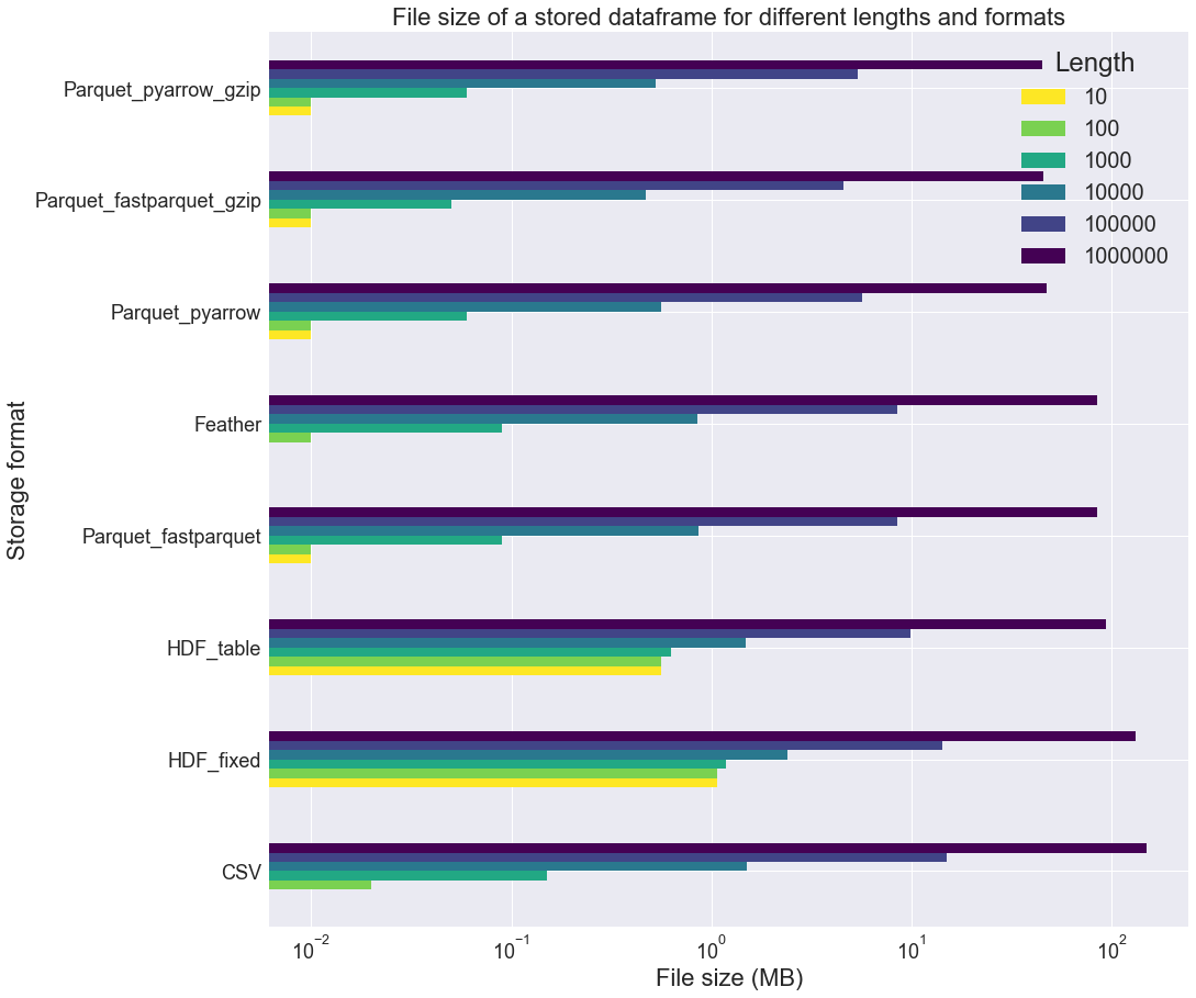
It appears that the Parquet_fastparquet_gzip, Parquet_pyarrow_gzip and Parquet_pyarrow formats are rather compact. HDF formats seems rather inadequate when dealing with small tables. The Parquet_pyarrow_gzip file is about 3 times smaller than the CSV one.
Also, note that many of these formats use equal or more space to store the data on a file than in memory (Feather, Parquet_fastparquet, HDF_table, HDF_fixed, CSV). This might be because the categorical columns are stored as str columns in the files, which is a redundant storage.
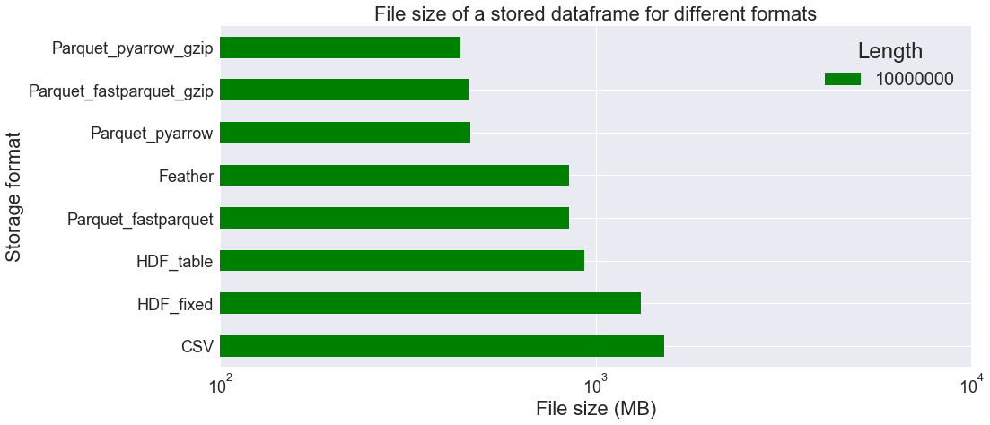
Now let us focus on longer tables in order to see whether HDF or Parquet performs better. We do not consider a DB storage anymore (tests are too long to perform, especially for data injection), but only single file storage. We set n=10000000 (memory usage of the dataframe: 810.629 MB).
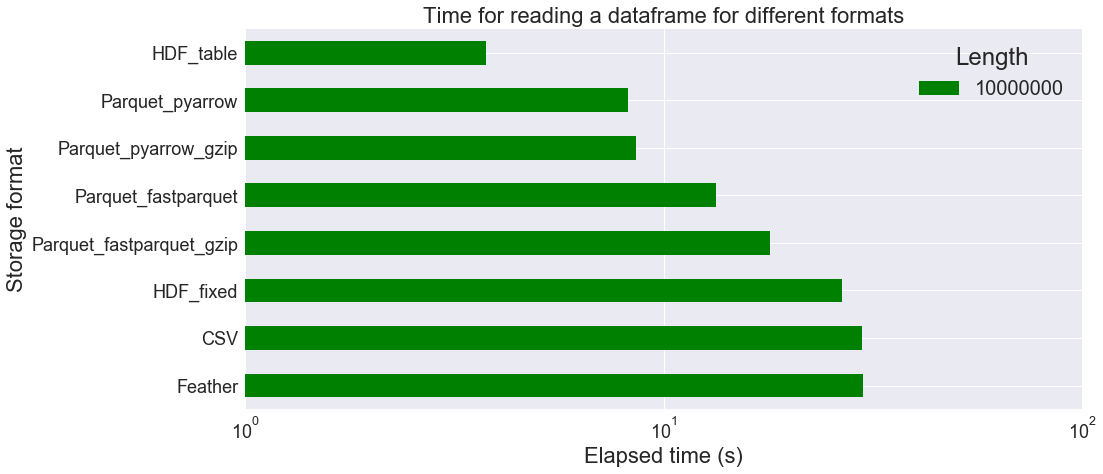
We observe above that HDF_table is faster than other file formats for longer tables, but this may be partly because we don’t have to convert the string columns back into the categorical type. At best, it only takes 3.77 s to load the data, instead of 29.80 s for CSV format (8.21 s for Parquet_pyarrow). On the other hand, file size is larger when using HDF_table (932.57 MB) than Parquet_pyarrow (464.13 MB). The CSV format file is is the largest: 1522.37 MB!
Loop on different widths
The table length n is now fixed (n=100000) and only the number of columns is changed, always with the same proportion of int, float and categorical columns (1/3 each). We start from 15 and increases the column count up to 150. Here are the results:
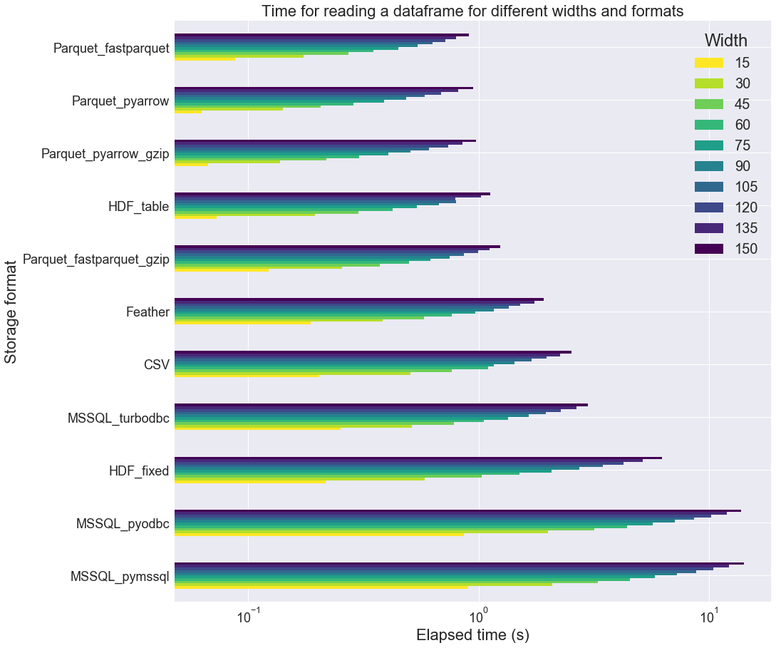
We can observe that Parquet_fastparquet behaves better with larger tables, as opposed to HDF_table. Parquet_pyarrow still is in the leading trio. Still, MSSQL_turbobdc outperforms the two other MSSQL drivers.
If we look at the file size, we note that HDF files are rather large as compared to Parquet_fastparquet_gzip or Parquet_pyarrow_gzip.
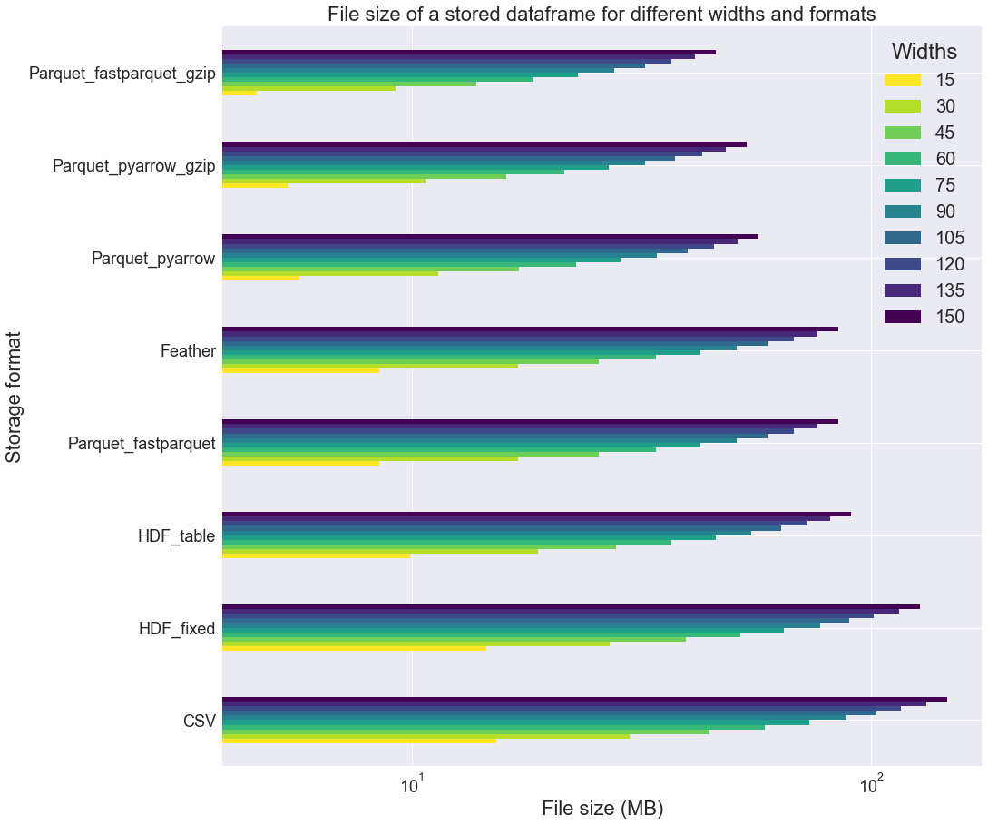
It seems that the gzip compression is really more effective when applied to Parquet_fastparquet than Parquet_pyarrow, for which it is almost useless.
Loop on different entropies
For this section, we are just going to look at the elapsed time (not the file size). The table length n is still fixed (n=100000), as well as the number of columns: 100 (n_int=50, n_float=0, n_str=50). Only the “entropy coefficient” e does vary betwen 0 and 1000. e is related to the number of unique values in each column in the following way: i_max = 50 + e and n_cat = 10 + e.
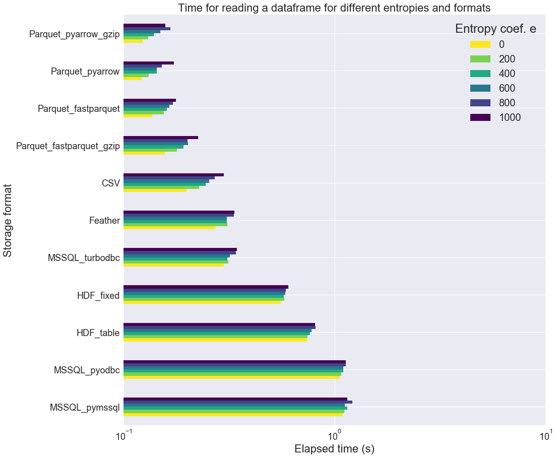
From the above figure, it seems that the “entropy coef” has a very small influence on the loading time for most of the formats. Surprisingly, it does have some kind of influence on the reading time of CSV files. It also have a non-negligible influence on all the Parquet formats.
Conclusion
It is important to stress that we are not dealing here with big data processing, but rather very common small to medium size datasets. Here is what we can get from this performance study:
- Parquet_pyarrow is a good choice in most cases regarding both loading time and disk space
- HDF_table is the fastest format when dealing with larger datasets.
- MSSQL_turbobdc is rather efficient as compared to other MSSQL drivers, achieving similar timings as the CSV file format
Please drop a comment if ever you think something in this post is not clear or inaccurate!