Fetching AROME weather forecasts and plotting temperatures
Accurate weather forecasts might be very usefull for various types of models. In this post, we are going to download the latest available weather forecasts for France and plot some temperature fields, using different Python libraries:
Arome is small scale numerical prediction model, operational at Meteo-France. AROME forecasts are available on the Meteo-France website here under the ETALAB licence.
![]()
From what we understand they only have been made available as “open data” since July 2019. The data files from Meteo-France are available as grib2 files. We are going to use the simple pygrib package to read them. Here is a summary of what we are going to do in this post:
- download the latest forecasts
- open the grib2 files
- get the spatial grid
- stack the temperature files into a 3D Numpy array
- get a background map
- plot the temperature fields
Let us start by importing a few libraries (we use CPython 3.7.6 on a Linux OS):
import os, sys
import datetime
import subprocess

import pygrib
import matplotlib.pyplot as plt
import numpy as np
import pandas as pd
import geopandas as gpd
from shapely.geometry import Point, Polygon
Download the latest forecasts
The first thing we need to do is guessing the latest available run from Meteo France. In order to do that, we have the following function inspired from this repo:
def get_latest_run_time(delay=4):
    ''' Runs are updated at 0am, 3am, 6am, 0pm, 6pm UTC.
        Note that the delay must be adjusted.
    '''
    utc_now = datetime.datetime.utcnow()
    candidate = datetime.datetime(utc_now.year, utc_now.month, utc_now.day, utc_now.hour) - \
        datetime.timedelta(hours=delay)
    run_time = datetime.datetime(candidate.year, candidate.month, candidate.day)
    for hour in np.flip(np.sort([3, 6, 12, 18])):
        if candidate.hour >= hour:
            run_time += datetime.timedelta(hours=int(hour))
            break
    return run_time.isoformat()

run_time = get_latest_run_time()
print(run_time)
2020-01-20T06:00:00
So the latest available results from the AROME model dates back from today at 6am UTC. We are going to build the URL where the files can be fetched. Next, we need to define the forecasting time range(s) that we interested in. The available time ranges are the following ones: 0-6H, 7-12H, 13-18H, 19-24H, 25-30, 31-36H and 37-42H. The time range string is returned by the following function given an int between 0 and 6:
def get_time_range(batch_number=0):
    ''' 7 different 6-hours long time ranges: 0-6H, 7-12H, ... , 37-42H.
    '''
    assert batch_number in range(7)
    end = 6 * (batch_number + 1)
    if batch_number == 0:
        start = 0
    else:
        start = end - 5
    time_range = str(start).zfill(2) + 'H' + str(end).zfill(2) +'H'
    return time_range

time_range = get_time_range(3)
time_range
'19H24H'
Let’s say we are interested in all the different time ranges, and gather them into a list:
time_ranges = []
for batch_number in range(7):
    time_ranges.append(get_time_range(batch_number))
time_ranges
['00H06H', '07H12H', '13H18H', '19H24H', '25H30H', '31H36H', '37H42H']
Now we are going to use 2 functions returning strings:
- one to create the URLs
- one to create the path where each file is going to be saved
One of the parameter of these functions is package: this defines a group of weather fields. We are going to fetch the SP1 package, which contains “current surface parameters”, and specifically the surface temperature. Also, we are going to fetch the results with a 0.025° resolution. We tried the finer ones (0.01°) but did not succeed in opening the files in Python, but only with the XyGrib software. Note that 11 different packages are available on the Meteo-France web site with the coarser resolution (0.025°).
def create_url(run_time, time_range='00H06H', package='SP1', token='__5yLVTdr-sGeHoPitnFc7TZ6MhBcJxuSsoZp6y0leVHU__'):
    ''' This creates the url string to get the data with 0.025° spatial accuracy.
    '''
    assert package in ['HP1', 'HP2', 'HP3', 'IP1', 'IP2', 'IP3', 'IP4', 'IP5', 'SP1', 'SP2', 'SP3']
    url = f'http://dcpc-nwp.meteo.fr/services/PS_GetCache_DCPCPreviNum\?token\={token}' \
    + f'\&model\=AROME\&grid\=0.025\&package\={package}\&time\={time_range}\&referencetime\={run_time}Z\&format\=grib2'
    return url

def create_file_name(run_time, time_range='00H06H', package='SP1'):
    dt = ''.join(run_time.split(':')[0:2]).replace('-', '').replace('T', '')
    file_name = f'AROME_0.025_{package}_{time_range}_{dt}.grib2'
    return file_name
We can now build a list of all URLs and target file names:
files = []
for time_range in time_ranges:
    url = create_url(run_time, time_range)
    file_name = create_file_name(run_time, time_range)
    file_path = os.path.join(os.getcwd(), file_name)  # files are downloaded locally
    cmd = f'wget --output-document {file_path} {url}'
    files.append({'url': url, 'file_name': file_name, 'file_path': file_path, 'cmd': cmd})
files[0]  # let's display the first item from the list
{'url': 'http://dcpc-nwp.meteo.fr/services/PS_GetCache_DCPCPreviNum\\?token\\=__5yLVTdr-sGeHoPitnFc7TZ6MhBcJxuSsoZp6y0leVHU__\\&model\\=AROME\\&grid\\=0.025\\&package\\=SP1\\&time\\=00H06H\\&referencetime\\=2020-01-20T06:00:00Z\\&format\\=grib2',
 'file_name': 'AROME_0.025_SP1_00H06H_202001200600.grib2',
 'file_path': '/home/francois/Workspace/AROME/AROME_0.025_SP1_00H06H_202001200600.grib2',
 'cmd': 'wget --output-document /home/francois/Workspace/AROME/AROME_0.025_SP1_00H06H_202001200600.grib2 http://dcpc-nwp.meteo.fr/services/PS_GetCache_DCPCPreviNum\\?token\\=__5yLVTdr-sGeHoPitnFc7TZ6MhBcJxuSsoZp6y0leVHU__\\&model\\=AROME\\&grid\\=0.025\\&package\\=SP1\\&time\\=00H06H\\&referencetime\\=2020-01-20T06:00:00Z\\&format\\=grib2'}
Next we download the data files sequentially.
%%time
for cmd in [file['cmd'] for file in files]:
    subprocess.call(cmd, shell=True)
CPU times: user 51.2 ms, sys: 66.1 ms, total: 117 ms
Wall time: 28min 26s
28 min is quite long! This could be easily parallelized but is the upstream server allowing multiple requests from the same IP? Anyway we (slowly) got the following files:
!ls -s *.grib2
31808 AROME_0.025_SP1_00H06H_202001200600.grib2
29268 AROME_0.025_SP1_07H12H_202001200600.grib2
29692 AROME_0.025_SP1_13H18H_202001200600.grib2
29712 AROME_0.025_SP1_19H24H_202001200600.grib2
30552 AROME_0.025_SP1_25H30H_202001200600.grib2
29928 AROME_0.025_SP1_31H36H_202001200600.grib2
    0 AROME_0.025_SP1_37H42H_202001200600.grib2
We can notice that the last file was not available from the Meteo-France server at the moment we tried to access it. Also, we can observe that the files aren’t so large (around 30 MB each).
Open the grib2 files
We use the handy pygrib package:
grbs = []
for item in files:
    grbs.append(pygrib.open(item['file_path']))
Also, we get all the description data and gather them into a dataframe:
descr = []
for item in grbs:
    item.seek(0)
    for grb in item:
        descr.append(str(grb).split(':'))
df = pd.DataFrame(
    descr,
    columns=['id', 'name', 'unit', 'spacing', 'layer', 'level', 'hour', 'run_dt'])
df.head(2)
| id | name | unit | spacing | layer | level | hour | run_dt | |
|---|---|---|---|---|---|---|---|---|
| 0 | 1 | Mean sea level pressure | Pa (instant) | regular_ll | meanSea | level 0 | fcst time 0 hrs | from 202001200600 |
| 1 | 2 | Mean sea level pressure | Pa (instant) | regular_ll | meanSea | level 0 | fcst time 1 hrs | from 202001200600 |
len(df)
547
We actually have 547 layers. Let us look at the different fields found in the files:
df.name.unique()
array(['Mean sea level pressure', '10 metre U wind component',
       '10 metre V wind component', '10 metre wind direction',
       '10 metre wind speed', 'Wind speed (gust)',
       'u-component of wind (gust)', 'v-component of wind (gust)',
       '2 metre temperature', '2 metre relative humidity',
       'Total Precipitation', 'Snow melt',
       'Downward short-wave radiation flux', '75', 'Total Cloud Cover'],
      dtype=object)
Obviously, not all the 15 variables are available for each of the 37 hours, or we would have 555 layers. This is because some of the variables do not exhibit the same one-hour based temporality. Let’s look at the 2 metre temperature variable:
df.loc[df.name == '2 metre temperature', 'hour'].values
array(['fcst time 0 hrs', 'fcst time 1 hrs', 'fcst time 2 hrs',
       'fcst time 3 hrs', 'fcst time 4 hrs', 'fcst time 5 hrs',
       'fcst time 6 hrs', 'fcst time 7 hrs', 'fcst time 8 hrs',
       'fcst time 9 hrs', 'fcst time 10 hrs', 'fcst time 11 hrs',
       'fcst time 12 hrs', 'fcst time 13 hrs', 'fcst time 14 hrs',
       'fcst time 15 hrs', 'fcst time 16 hrs', 'fcst time 17 hrs',
       'fcst time 18 hrs', 'fcst time 19 hrs', 'fcst time 20 hrs',
       'fcst time 21 hrs', 'fcst time 22 hrs', 'fcst time 23 hrs',
       'fcst time 24 hrs', 'fcst time 25 hrs', 'fcst time 26 hrs',
       'fcst time 27 hrs', 'fcst time 28 hrs', 'fcst time 29 hrs',
       'fcst time 30 hrs', 'fcst time 31 hrs', 'fcst time 32 hrs',
       'fcst time 33 hrs', 'fcst time 34 hrs', 'fcst time 35 hrs',
       'fcst time 36 hrs'], dtype=object)
All the 37 hours are found.
Get the spatial grid
Here we look for the first temperature field and get the associated grid:
grb = grbs[0][54]
grb
54:2 metre temperature:K (instant):regular_ll:heightAboveGround:level 2 m:fcst time 0 hrs:from 202001200600
lats, lons = grb.latlons()  # WGS84 projection
lats.shape, lats.min(), lats.max(), lons.shape, lons.min(), lons.max()
((601, 801), 38.00000000000085, 53.0, (601, 801), -8.0, 12.00000000000015)
So we assume that the grid is a uniform Catesian 801 x 601 grid.
shape = lats.shape
x = np.linspace(lons.min(), lons.max(), shape[1])
y = np.linspace(lats.min(), lats.max(), shape[0])
X, Y = np.meshgrid(x, y)
We also compute a ratio for the figure size:
ratio = (lats.max() - lats.min()) / (lons.max() - lons.min())
size_int = 20
fig_size = (size_int, int(round(ratio * size_int)))
fig_size
(20, 15)
Stack the temperature files into a 3D Numpy array
For each temperature layer, we extract the values as a NumPy array. The data is reverted along the 1st axis in order to be displayed correctly. Also, the temperature unit is changed from Kelvin to Celsius:
arrays = []
for batch_number in range(6):
    grb_hours = grbs[batch_number].select(name='2 metre temperature')
    for idx in range(len(grb_hours)):
        grb = grb_hours[idx]
        temper = np.copy(grb.values[::-1,])  # revert first axis
        temper -= 273.15  # from Kelvin to Celsius
        arrays.append(temper)
temperatures = np.stack(arrays, axis=2)
temperatures.shape
(601, 801, 37)
We can see that the 3rd dimension is the temporal one. We also compute the global min and max temperature in order to have a fixed colormap:
temp_min, temp_max = int(np.floor(np.min(temperatures))), int(np.ceil(np.max(temperatures)))
print(f'min {temp_min} / max {temp_max}')
min -31 / max 18
Get a background map
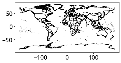
We would like to plot the temperature as filled contours on top of an administrative map, so that the different borders can be seen. The borders are loaded with GeoPandas from a shapefile found on the naturalearthdata.com web site. However these are all the countries in the world and we are only interested in a bounding box around France defined by the previous spatial grid.
# https://www.naturalearthdata.com/downloads/10m-cultural-vectors/10m-admin-0-countries/
world = gpd.read_file('./countries/ne_10m_admin_0_countries.shp')
ax = world.plot(color='white', edgecolor='black')
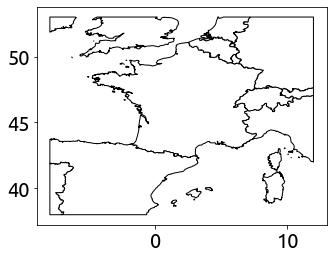
So let’s create a bounding box as a GeoDataFrame and intersect it with the world countries’ one:
p1 = Point(lons.min(), lats.min())
p2 = Point(lons.max(), lats.min())
p3 = Point(lons.max(), lats.max())
p4 = Point(lons.min(), lats.max())
np1 = (p1.coords.xy[0][0], p1.coords.xy[1][0])
np2 = (p2.coords.xy[0][0], p2.coords.xy[1][0])
np3 = (p3.coords.xy[0][0], p3.coords.xy[1][0])
np4 = (p4.coords.xy[0][0], p4.coords.xy[1][0])

bb_polygon = Polygon([np1, np2, np3, np4])
bbox = gpd.GeoDataFrame(geometry=[bb_polygon])
france = gpd.overlay(world, bbox, how='intersection')
france.plot(color='white', edgecolor='black');
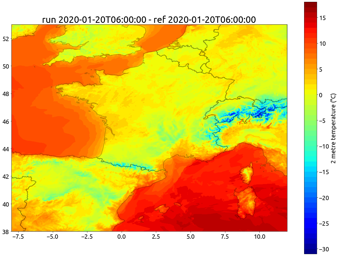
Plot the temperature fields
Here we go! Now we can finally plot the temperature fields:
creation_time = datetime.datetime.strptime(run_time, "%Y-%m-%dT%H:%M:%S")
movie = False
for k in range(temperatures.shape[2]):
    fig, ax = plt.subplots(figsize=fig_size)
    CS = ax.contourf(X, Y, temperatures[:,:,k], levels=np.arange(temp_min, temp_max + 1), cmap='jet');
    france.geometry.boundary.plot(ax=ax, color=None, edgecolor='k',linewidth=2, alpha=0.25);
    reference_time = creation_time + datetime.timedelta(hours=k)
    ax.set_title(f"run {creation_time.isoformat()} - ref {reference_time.isoformat()}");
    cbar = fig.colorbar(CS)
    cbar.ax.set_ylabel('2 metre temperature (°C)');
    if movie:
#         plt.savefig(f'temperature_{str(k).zfill(2)}.png', dpi=30) # low res
        plt.savefig(f'temperature_{str(k).zfill(2)}.png')  # high res
    else
        break
And this is the command line used to create the animated gif from all the png files (generated with movie = True):
# !convert -delay 10 -loop 0 temperature*.png animation.gif