A Quick study of air quality in Lyon with Python
The aim of this post is to use Python to fetch air quality data from a web service and to create a few plots.
We are going to:
- look at some daily data from earlier this year, before and after the lockdown, in the city of Lyon, France
- compare 2020 with some from previous years
- and eventually look at some specific pollutants
The data is provided by an organization called Atmo Auvergne-Rhône-Alpes monitoring air quality over the Auvergne-Rhône-Alpes region. They also come up with a convenient web API (HTTP GET method). Note that an API token is required, you can easily get from their website after registration.
Imports
from datetime import datetime

import requests
import pandas as pd
from fastprogress.fastprogress import progress_bar
from matplotlib import pyplot as plt

plt.style.use("seaborn")
%load_ext lab_black

FS = (16, 9)  # figure size

# location: LYON 4EME ARRONDISSEMENT (4th district)
CODE_INSEE = 69384

# api-token
API_TOKEN = "8xxxxxxxxxxxxxxxxxxxxxxxxxxxxxx7"

# api-endpoint
URL = f"https://api.atmo-aura.fr/communes/{CODE_INSEE}/indices?api_token={API_TOKEN}"
First try of the API
PARAMS = {"date": "2020-05-24"}
r = requests.get(url=URL, params=PARAMS)
data = r.json()
data
{'licence': 'https://opendatacommons.org/licenses/odbl/',
 'commune': 'LYON-4E-ARRONDISSEMENT',
 'code_insee': '69384',
 'indices': {'date': '2020-05-24',
  'valeur': '37.5560109609897',
  'couleur_html': '#99E600',
  'qualificatif': 'Bon',
  'type_valeur': 'prévision'}}
Since we will not change the location (4th district in Lyon), we only need to keep the date and valeur items from this dictionary. valeur is the air pollution index value. It ranges from 0 to 100, but could also rise above 100, which would mean that the warning threshold is exceeded. This would imply a serious risk to the population and the environment justifying the implementation of emergency measures.
Note that you can get historic values but also forecasts if you enter a future date in the get params (2 day horizon at most when I tried that).
So let’s fetch the daily pollution index on a temporal range starting at the begining of 2020 and ending today.
Daily air quality in 2020 so far
First we create a date range:
start = datetime(2020, 1, 1).date()
end = datetime.now().date()
day_range = pd.date_range(start=start, end=end, freq="D")
Now we can loop on these days and fetch the air quality data for each day. Since each item in day_range is a Timestamp object, we convert them to str with strftime:
daily_pollution_index = []
for day in progress_bar(day_range):
    day_str = day.strftime("%Y-%m-%d")
    params = {"date": day_str}
    r = requests.get(url=URL, params=params)
    data = r.json()
    daily_pollution_index.append(data["indices"])
The list is given to Pandas to create a dataframe:
df = pd.DataFrame(daily_pollution_index)
df.head(2)
| date | valeur | couleur_html | qualificatif | type_valeur | |
|---|---|---|---|---|---|
| 0 | 2020-01-01 | 50.4253716534476 | #FFFF00 | Moyen | réelle |
| 1 | 2020-01-02 | 48.5803761861679 | #C3F000 | Bon | réelle |
We clean up the dataframe a little bit, and create a DatetimeIndex:
df.rename(
    columns={"valeur": "value",}, inplace=True,
)
df.drop(["type_valeur", "couleur_html", "qualificatif"], axis=1, inplace=True)
df["value"] = df["value"].astype(float)
df["date"] = pd.to_datetime(df["date"])
df.set_index("date", inplace=True)
df.head(2)
| value | |
|---|---|
| date | |
| 2020-01-01 | 50.425372 |
| 2020-01-02 | 48.580376 |
And we can now plot the daily historical air pollution index.
ax = df["value"].plot(
    ms=10, linewidth=3, alpha=0.7, style="o-", figsize=FS, c="#1f77b4",
)
_ = plt.vlines("2020-03-17", 0, 100, colors="r")  # lockdown start
_ = plt.vlines("2020-05-11", 0, 100, colors="r")  # lockdown end
_ = ax.set_ylim(0, 100)
_ = ax.set(
    title="Daily air quality in Lyon 4E",
    xlabel="Date",
    ylabel="Air pollution index (smaller is better)",
)
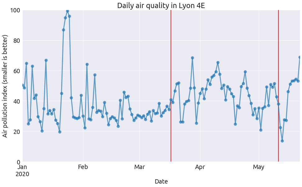
Well we do not see a significant drop in air pollution during the lockdown that took place between march 17 and may 11. The reason is that the air pollution index is combining 3 different kinds of pollutants:
- NO2: Nitrogen dioxide,
- O3: Ozone,
- PM10: particulate matter, which are coarse particles with a diameter between 2.5 and 10 micrometers (μm)
From what I understand, an index is computed for each of these three pollutants, and the air pollution index corresponds to a combination of these three values. So the pollution index will keep being large if any of these pollutant concentrations remain large.
Now theses pollutants have very different origins: NO2 is mainly related to road traffic and other fossil fuel combustion processes, PM10 to wood heating (in the suburb), agriculture,… O3 is more complex; here is a quote from wikipedia:
Ozone precursors are a group of pollutants, predominantly those emitted during the combustion of fossil fuels. Ground-level ozone pollution (tropospheric ozone) is created near the Earth’s surface by the action of daylight UV rays on these precursors. The ozone at ground level is primarily from fossil fuel precursors, but methane is a natural precursor, and the very low natural background level of ozone at ground level is considered safe.
And of course these levels of pollution also depends on the weather conditions. A cold weather may yield a larger PM10 concentration due to heating. A sunny weather may increase the level of ozone concentration, while some rain may “clean” the particles, I guess. So many factors contribute to air pollution.
Concerning the first part of 2020, let’s try to compare the above pollution values with the ones recorded in the 2 previous years.
Monthly air quality from 2018 to 2020
We already have the data for 2020, so we now fetch the data for the same range of days (january 1 to may 22), but for 2018 and 2019. The data from previous years (<2018) does not seem to be available on the web service.
daily_pollution_index = []
for year in range(2018, 2020):
    for day in progress_bar(day_range):
        try:
            day = day.replace(year=year).date()
            day_str = day.strftime("%Y-%m-%d")
            params = {"date": day_str}
            r = requests.get(url=URL, params=params)
            data = r.json()
            if data is not None:
                if data["indices"] is not None:
                    daily_pollution_index.append(data["indices"])
        except:
            print(f"No data for the date: {day.date()}")
No data for the date: 2020-02-29
No data for the date: 2020-02-29
Similarly to what we did before, we create a dataframe with a DatetimeIndex:
df_hist = pd.DataFrame(daily_pollution_index)
df_hist.rename(
    columns={"valeur": "value",}, inplace=True,
)
df_hist.drop(["type_valeur", "couleur_html", "qualificatif"], axis=1, inplace=True)
df_hist["value"] = df_hist["value"].astype(float)
df_hist["date"] = pd.to_datetime(df_hist["date"])
df_hist.set_index("date", inplace=True)
df_hist.head(2)
| value | |
|---|---|
| date | |
| 2018-01-01 | 32.346865 |
| 2018-01-02 | 31.257633 |
And we merge the data corresponding to the 3 different years:
df.rename(
    columns={"value": "2020",}, inplace=True,
)
df["month"] = df.index.month
df["day"] = df.index.day
df.reset_index(drop=False, inplace=True)
df_hist["month"] = df_hist.index.month
df_hist["day"] = df_hist.index.day
df_all = pd.merge(df, df_hist["2018"], on=["month", "day"], how="left").rename(
    columns={"value": "2018"}
)
df_all = pd.merge(df_all, df_hist["2019"], on=["month", "day"], how="left").rename(
    columns={"value": "2019"}
)
df_all.drop(["month", "day"], axis=1, inplace=True)
df_all.set_index("date", inplace=True)
df_all.head(2)
| 2020 | 2018 | 2019 | |
|---|---|---|---|
| date | |||
| 2020-01-01 | 50.425372 | 32.346865 | 21.538545 |
| 2020-01-02 | 48.580376 | 31.257633 | 31.926375 |
Let’s plot the monthly average:
monthly = df_all.resample("M").mean()
monthly["month"] = monthly.index.month_name()
monthly.set_index("month", inplace=True, drop=True)
ax = monthly.plot.bar(figsize=FS, rot=10)
_ = ax.set_ylim(0, 100)
_ = ax.set(
    title="Monthly air quality in Lyon 4E",
    xlabel="Date",
    ylabel="Air pollution index (smaller is better)",
)
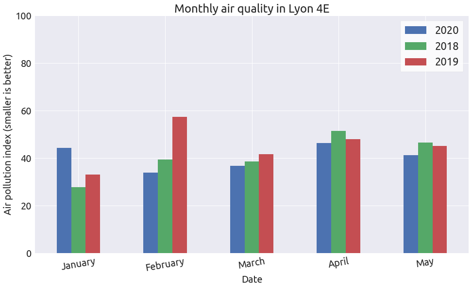
Well there is no significant difference between the different years.
Unfortunately the web service does not offer separate data for each pollutant. However these data are available from their website here, as CSV files.
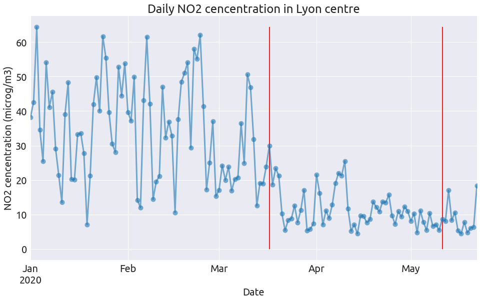
Daily concentration of 3 pollutants
We download the data for the 3 pollutants seen earlier, on the same time range and with the same frequency. Let’s look at the first file:
NO2 = pd.read_csv("NO2.csv", sep=";")
NO2
| Station | Polluant | Mesure | Unité | 01/01/2020 | ... | 22/05/2020 | |
|---|---|---|---|---|---|---|---|
| 0 | Lyon Centre | Dioxyde d'azote | Dioxyde d'azote | microg/m3 | 38,2 | ... | 18,3 |
1 rows × 147 columns
We need to transpose the dataframe in order to create a DatetimeIndex, and take care of the french number and date formats:
NO2.drop(["Station", "Polluant", "Mesure", "Unité"], axis=1, inplace=True)
NO2 = NO2.T
NO2.index = pd.to_datetime(NO2.index, format="%d/%m/%Y")
NO2.columns = ["NO2"]
NO2["NO2"] = NO2["NO2"].astype(str).map(lambda s: s.replace(",", ".")).astype(float)
NO2.head(2)
| NO2 | |
|---|---|
| 2020-01-01 | 38.2 |
| 2020-01-02 | 42.6 |
Now we do the same with the two other files and concatenate the 3 columns:
O3 = pd.read_csv("O3.csv", sep=";")
O3.drop(["Station", "Polluant", "Mesure", "Unité"], axis=1, inplace=True)
O3 = O3.T
O3.index = pd.to_datetime(O3.index, format="%d/%m/%Y")
O3.columns = ["O3"]
O3["O3"] = O3["O3"].astype(str).map(lambda s: s.replace(",", ".")).astype(float)
PM10 = pd.read_csv("PM10.csv", sep=";")
PM10.drop(["Station", "Polluant", "Mesure", "Unité"], axis=1, inplace=True)
PM10 = PM10.T
PM10.index = pd.to_datetime(PM10.index, format="%d/%m/%Y")
PM10.columns = ["PM10"]
PM10["PM10"] = PM10["PM10"].astype(str).map(lambda s: s.replace(",", ".")).astype(float)
pol = pd.concat([NO2, O3, PM10], axis=1)
pol.head(2)
| NO2 | O3 | PM10 | |
|---|---|---|---|
| 2020-01-01 | 38.2 | 0.8 | 38.2 |
| 2020-01-02 | 42.6 | 0.9 | 35.1 |
Here is a little function to plot each pollutant:
def plot_pollutant(df, pollutant, unit):
    ax = pol[pollutant].plot(
        ms=10,
        linewidth=3,
        alpha=0.6,
        style="-o",
        legend=False,
        color=colors[0],
        figsize=FS,
    )
    max_val = pol[pollutant].max()
    _ = plt.vlines("2020-03-17", 0, max_val, colors="r")  # lockdown start
    _ = plt.vlines("2020-05-11", 0, max_val, colors="r")  # lockdown end
    _ = ax.set(
        title=f"Daily {pollutant} cencentration in Lyon centre",
        xlabel="Date",
        ylabel=f"{pollutant} cencentration ({unit})",
    )
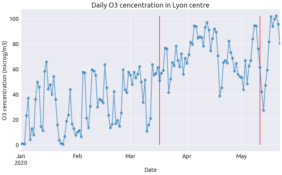
that we can call 3 times:
plot_pollutant(pol, "NO2", "microg/m3")
plot_pollutant(pol, "O3", "microg/m3")
plot_pollutant(pol, "PM10", "microg/m3")
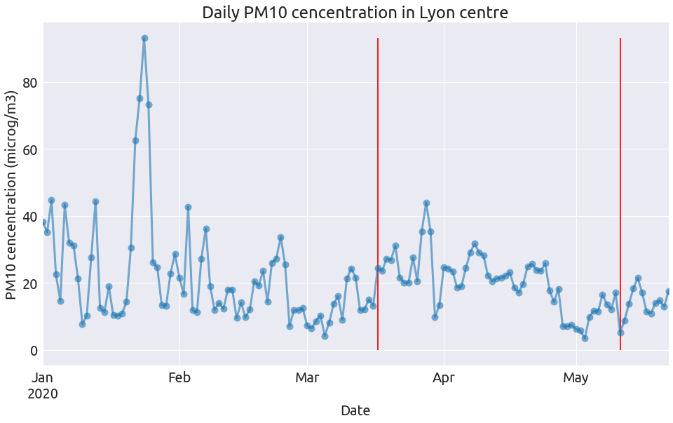
So clearly the NO2 concentration dropped at the begining of the lockdown alongside the intensity of road traffic, and remain low after (as does road traffic). The level of the two other pollutants during lockdown have a lot do with the specific weather conditions (see this page from Atmo).