Minimizing continuous non-convex functions with Optuna

In this post, we are going to deal with single-objective continuous optimization problems, using the open-source Optuna Python package. Here is a very short description of this library from their github repository:

Optuna is an automatic hyperparameter optimization software framework, particularly designed for machine learning. It features an imperative, define-by-run style user API. Thanks to our define-by-run API, the code written with Optuna enjoys high modularity, and the user of Optuna can dynamically construct the search spaces for the hyperparameters.

Optuna is a really great package for HyperParameter Optimization (HPO). I have been using it for a little while along several machine learning frameworks such as XGBoost, LightGBM, Scikit-Learn, Keras, etc… Optuna is powerful, efficient and easy to use. From what I understand, it is developped by the people from the japanese company Preferred Networks Inc, which brought some other great open-source packages such as Chainer or CuPy.

Let’s use it here on some “textbook” optimization problems, minimizing 4 classic non-convex test functions for single-objective optimization:

• Rastrigin
• Ackley
• Rosenbrock
• Himmelblau

We are going to use the Covariance matrix adaptation evolution strategy (CMA-ES) algorithm, which is an evolutionary strategy (stochastic, derivative-free) available in Optuna as optuna.samplers.CmaEsSampler. Note that this sampler does not support categorical distributions in case you would like to use it for HPO.

Imports

import numpy as np
from mpl_toolkits import mplot3d
import matplotlib.pyplot as plt
from numba import jit
import optuna

# suppress log messages from Optuna
optuna.logging.set_verbosity(optuna.logging.WARNING)

%load_ext watermark

SD = 123  # random seed

%watermark

2020-08-28T16:03:01+02:00

CPython 3.8.5
IPython 7.17.0

compiler   : GCC 7.5.0
system     : Linux
release    : 4.15.0-112-generic
machine    : x86_64
processor  : x86_64
CPU cores  : 8
interpreter: 64bit

%watermark --iversions

matplotlib 3.3.1
optuna     2.0.0
numpy      1.19.1

Note that Optuna 2.0 was just realeased last month.

Early stopping callback

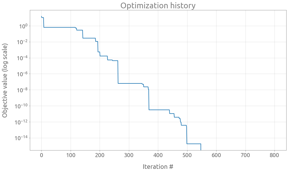
An assumption in the following is that we do not know the minimum value of the objective function. This is why we create a stopping criterion in which an EarlyStoppingExceeded exception is raised when the score does not decrease in OPTUNA_EARLY_STOPING successive iterations. I found this implementation of early stopping callback on github here (nicely provided by https://github.com/Alex-Lekov).

OPTUNA_EARLY_STOPING = 250  # number of stagnation iterations required to raise an EarlyStoppingExceeded exception


class EarlyStoppingExceeded(optuna.exceptions.OptunaError):
    early_stop = OPTUNA_EARLY_STOPING
    early_stop_count = 0
    best_score = None


def early_stopping_opt(study, trial):
    if EarlyStoppingExceeded.best_score == None:
        EarlyStoppingExceeded.best_score = study.best_value

    if study.best_value < EarlyStoppingExceeded.best_score:
        EarlyStoppingExceeded.best_score = study.best_value
        EarlyStoppingExceeded.early_stop_count = 0
    else:
        if EarlyStoppingExceeded.early_stop_count > EarlyStoppingExceeded.early_stop:
            EarlyStoppingExceeded.early_stop_count = 0
            best_score = None
            raise EarlyStoppingExceeded()
        else:
            EarlyStoppingExceeded.early_stop_count = (
                EarlyStoppingExceeded.early_stop_count + 1
            )
    return

Rastrigin function

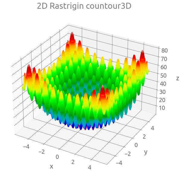
The Rastrigin is a non-linear multi-modal function. Here is the formula of the Rastrigin function:

$f(\mathbf{x}) = A n + \sum_{i=1}^n \left[ x_i^2 - A \cos(2 \pi x_i) \right],$

where $A=10$.

We are going to use only a 2-dimensional version of the function ($n=2$):

@jit(nopython=True)
def rastrigin_2D(x, y, A=10):
    return (
        2 * A
        + (np.square(x) - A * np.cos(2 * np.pi * x))
        + (np.square(y) - A * np.cos(2 * np.pi * y))
    )

The search domain is $-5.12 \leq x_i \leq 5.12$, for $i=1, 2$.

Plots

N = 100
x = np.linspace(-5.12, 5.12, N)
y = np.linspace(-5.12, 5.12, N)

X, Y = np.meshgrid(x, y)
Z = rastrigin_2D(X, Y)

fig = plt.figure(figsize=(10, 10))
ax = plt.axes(projection="3d")
ax.contour3D(X, Y, Z, 150, cmap="nipy_spectral")
_ = ax.set(xlabel="x", ylabel="y", zlabel="z", title="2D Rastrigin countour3D")

fig, ax = plt.subplots(figsize=(10, 8))
cs = plt.contourf(X, Y, Z, 150, cmap="nipy_spectral")
cb = fig.colorbar(cs, ax=ax, shrink=0.9)
_ = plt.plot(0, 0, "wo", ms=15)
_ = ax.set(xlabel="x", ylabel="y", title="2D Rastrigin countourf")

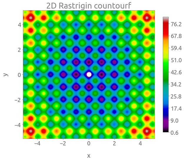
The global minimum is located at $\mathbf{x} = (0, 0)$ where $f(\mathbf{x}) = 0$.

Optimization

# Optuna's objective function
def objective(trial):
    x = trial.suggest_uniform("x", -5.12, 5.12)
    y = trial.suggest_uniform("y", -5.12, 5.12)
    return rastrigin_2D(x, y)


# Optuna' Sampler
sampler = optuna.samplers.CmaEsSampler(seed=SD)

# Optuna' Study
study = optuna.create_study(sampler=sampler)

%%time
try:
    study.optimize(
        objective, n_trials=50000, timeout=600, callbacks=[early_stopping_opt]
    )
except EarlyStoppingExceeded:
    print(f"EarlyStopping Exceeded: No new best scores in {OPTUNA_EARLY_STOPING} iterations")

EarlyStopping Exceeded: No new best scores in 250 iterations
CPU times: user 1.18 s, sys: 0 ns, total: 1.18 s
Wall time: 1.2 s

study.best_params

{'x': -3.8548264908988565e-10, 'y': -5.211127394832204e-10}

study.best_value

0.0

trials = study.trials_dataframe()
trials.head(2)

	number	value	datetime_start	...	state
0	0	15.185858	2020-08-28 16:03:03.971095	...	COMPLETE
1	1	10.601259	2020-08-28 16:03:04.056077	...	COMPLETE

ax = trials.value.expanding().min().plot(logy=True, figsize=(16, 9))
ax.set(
    title="Optimization history",
    xlabel="Iteration #",
    ylabel="Objective value (log scale)",
)
ax.grid()

Ackley function

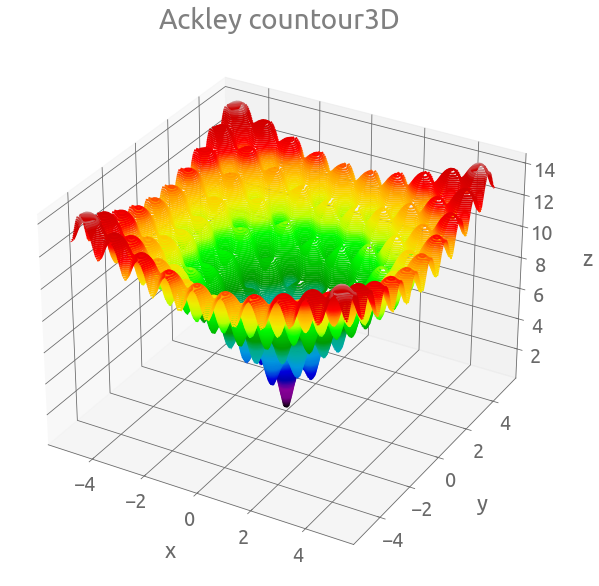
Here is the formula of Ackley function:

$f(x, y) = -20 \exp \left[-0.2 \sqrt{0.5 (x^2+y^2)} \right] - \exp \left[0.5 \left( \cos(2 \pi x) + \cos(2 \pi y) \right) \right] + e +20 $

@jit(nopython=True)
def ackley(x, y):
    return (
        -20 * np.exp(-0.2 * np.sqrt(0.5 * (np.square(x) + np.square(y))))
        - np.exp(0.5 * (np.cos(2 * np.pi * x) + np.cos(2 * np.pi * y)))
        + np.e
        + 20
    )

The search domain is $-5 \leq x, y \leq 5$.

Plots

N = 100
x = np.linspace(-5.0, 5.0, N)
y = np.linspace(-5.0, 5.0, N)

X, Y = np.meshgrid(x, y)
Z = ackley(X, Y)

fig = plt.figure(figsize=(10, 10))
ax = plt.axes(projection="3d")
ax.contour3D(X, Y, Z, 150, cmap="nipy_spectral")
_ = ax.set(xlabel="x", ylabel="y", zlabel="z", title="Ackley countour3D")

fig, ax = plt.subplots(figsize=(10, 8))
cs = plt.contourf(X, Y, Z, 150, cmap="nipy_spectral")
cb = fig.colorbar(cs, ax=ax, shrink=0.9)
_ = plt.plot(0, 0, "wo", ms=15)
_ = ax.set(xlabel="x", ylabel="y", title="Ackley countourf")

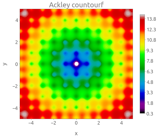
Again, the global minimum is located at $(x, y) = (0, 0)$ where $f(x, y) = 0$.

Optimization

# Optuna's objective function
def objective(trial):
    x = trial.suggest_uniform("x", -5.0, 5.0)
    y = trial.suggest_uniform("y", -5.0, 5.0)
    return ackley(x, y)


# Optuna' Sampler
sampler = optuna.samplers.CmaEsSampler(seed=SD)

# Optuna' Study
study = optuna.create_study(sampler=sampler)

# reset the EarlyStoppingExceeded class
EarlyStoppingExceeded.early_stop = OPTUNA_EARLY_STOPING
EarlyStoppingExceeded.early_stop_count = 0
EarlyStoppingExceeded.best_score = None

%%time
try:
    study.optimize(
        objective, n_trials=50000, timeout=600, callbacks=[early_stopping_opt]
    )
except EarlyStoppingExceeded:
    print(f"EarlyStopping Exceeded: No new best scores on iters {OPTUNA_EARLY_STOPING}")

EarlyStopping Exceeded: No new best scores on iters 250
CPU times: user 1.57 s, sys: 8.06 ms, total: 1.58 s
Wall time: 1.58 s

study.best_params

{'x': 2.604765386682313e-17, 'y': 2.52303410018247e-16}

study.best_value

0.0

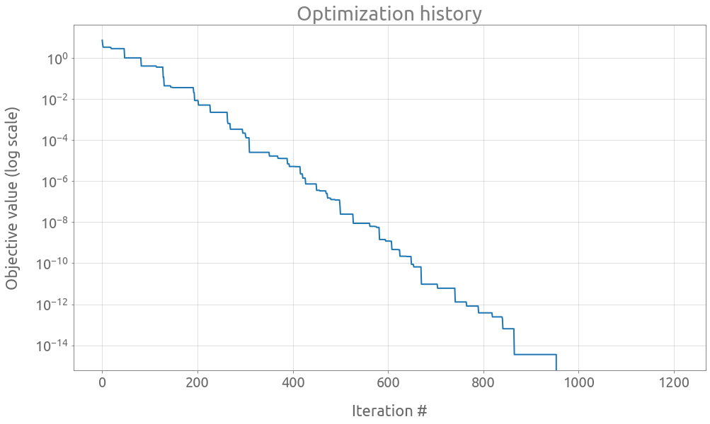
trials = study.trials_dataframe()
ax = trials.value.expanding().min().plot(logy=True, figsize=(16, 9))
ax.set(
    title="Optimization history",
    xlabel="Iteration #",
    ylabel="Objective value (log scale)",
)
ax.grid()

Rosenbrock function

As explained on the wikipedia page:

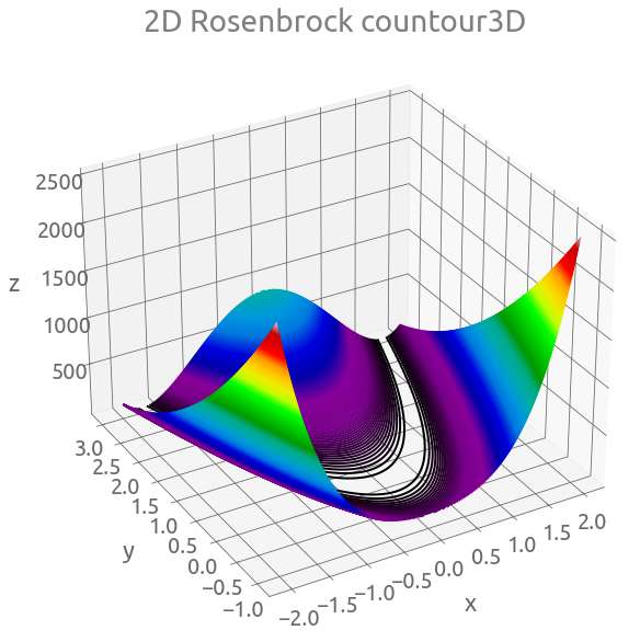
The global minimum is inside a long, narrow, parabolic shaped flat valley. To find the valley is trivial. To converge to the global minimum, however, is difficult.

Here is the formula:

$f( \mathbf{x}) = \sum_{i=1}^{n-1}\left[ 100 ( x_{i+1} - x_i^2)^2 + (1 - x_i)^2 \right],$

with $n \geq 2$. We are going to use only a 2-dimensional version of the function ($n=2$):

@jit(nopython=True)
def rosenbrock_2D(x, y):
    return np.square(1 - x) + 100 * np.square(y - np.square(x))

The search domain is $-\infty \leq x, y \leq \infty$. Let’s limit the domain to $[-10, 10]^2$ for the search space.

Plots

N = 100
x = np.linspace(-2, 2, N)
y = np.linspace(-1, 3, N)

X, Y = np.meshgrid(x, y)
Z = rosenbrock_2D(X, Y)

fig = plt.figure(figsize=(10, 10))
ax = plt.axes(projection="3d")
ax.view_init(30, -120)
ax.contour3D(X, Y, Z, 500, cmap="nipy_spectral")
_ = ax.set(xlabel="x", ylabel="y", zlabel="z", title="2D Rosenbrock countour3D")

fig, ax = plt.subplots(figsize=(10, 8))
cs = plt.contourf(X, Y, Z, 500, cmap="nipy_spectral")
cb = fig.colorbar(cs, ax=ax, shrink=0.9)
_ = plt.plot(1, 1, "wo", ms=15)
_ = ax.set(xlabel="x", ylabel="y", title="2D Rosenbrock countourf")

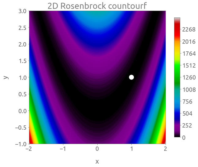
The global minimum is located at $(x, y) = (1, 1)$ where $f(x, y) = 0$.

Optimization

# Optuna's objective function
def objective(trial):
    x = trial.suggest_uniform("x", -10.0, 10.0)
    y = trial.suggest_uniform("y", -10.0, 10.0)
    return rosenbrock_2D(x, y)


# Optuna' Sampler
sampler = optuna.samplers.CmaEsSampler(seed=SD)

# Optuna' Study
study = optuna.create_study(sampler=sampler)

# reset the EarlyStoppingExceeded class
EarlyStoppingExceeded.early_stop = OPTUNA_EARLY_STOPING
EarlyStoppingExceeded.early_stop_count = 0
EarlyStoppingExceeded.best_score = None

%%time
try:
    study.optimize(
        objective, n_trials=50000, timeout=600, callbacks=[early_stopping_opt]
    )
except EarlyStoppingExceeded:
    print(f"EarlyStopping Exceeded: No new best scores on iters {OPTUNA_EARLY_STOPING}")

EarlyStopping Exceeded: No new best scores on iters 250
CPU times: user 1.92 s, sys: 11.6 ms, total: 1.93 s
Wall time: 1.93 s

study.best_params

{'x': 1.0, 'y': 1.0}

study.best_value

0.0

trials = study.trials_dataframe()
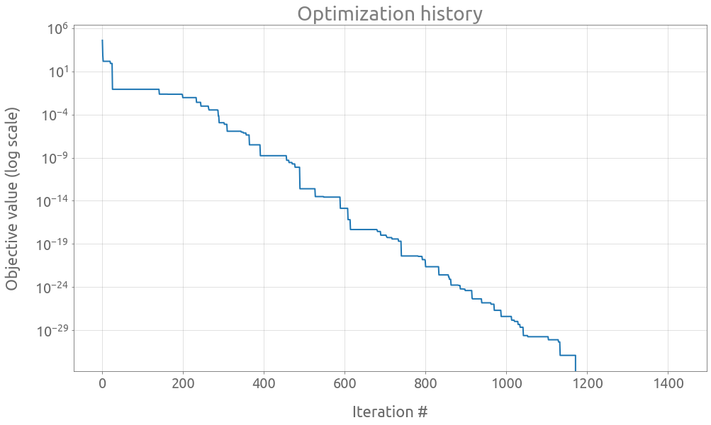
ax = trials.value.expanding().min().plot(logy=True, figsize=(16, 9))
ax.set(
    title="Optimization history",
    xlabel="Iteration #",
    ylabel="Objective value (log scale)",
)
ax.grid()

Himmelblau’s function

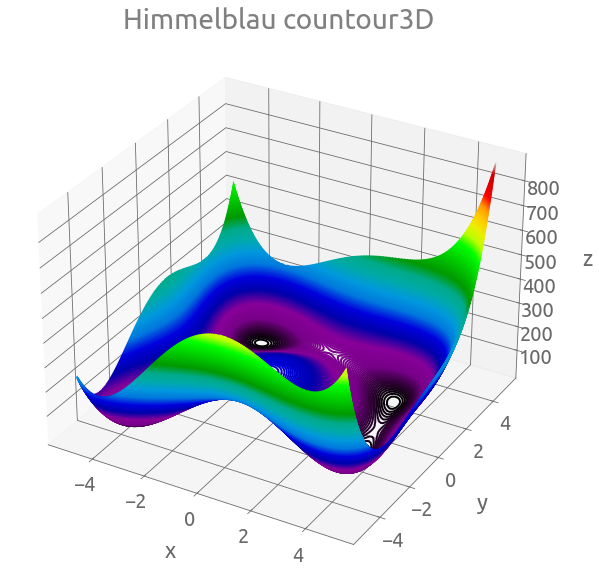
Himmelblau’s function is a 2D multi-modal function, with this formula:

$f(x,y)=(x^{2}+y-11)^{2}+(x+y^{2}-7)^{2}$.

@jit(nopython=True)
def himmelblau(x, y):
    return np.square(np.square(x) + y - 11) + np.square(x + np.square(y) - 7)

The search domain is $-\infty \leq x, y \leq \infty$. Let’s limit the domain to $[-5, 5]^2$ for the search space.

Plots

N = 100
x = np.linspace(-5, 5, N)
y = np.linspace(-5, 5, N)

X, Y = np.meshgrid(x, y)
Z = himmelblau(X, Y)

fig = plt.figure(figsize=(10, 10))
ax = plt.axes(projection="3d")
ax.contour3D(X, Y, Z, 500, cmap="nipy_spectral")
_ = ax.set(xlabel="x", ylabel="y", zlabel="z", title="Himmelblau countour3D")

fig, ax = plt.subplots(figsize=(10, 8))
cs = plt.contourf(X, Y, Z, 150, cmap="nipy_spectral")
cb = fig.colorbar(cs, ax=ax, shrink=0.9)
_ = plt.plot(3, 2, "wo", ms=15)
_ = plt.plot(-2.805118, 3.283186, "wo", ms=15)
_ = plt.plot(-3.779310, -3.283186, "wo", ms=15)
_ = plt.plot(3.584458, -1.848126, "wo", ms=15)
_ = ax.set(xlabel="x", ylabel="y", title="Himmelblau countourf")

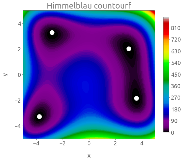
The Himmelblau function has four equal local minima $f(x, y) = 0$, located at:

• $(x, y) = (3, 2)$,
• $(x, y) = (-2.805118, 3.131312)$ (approx.),
• $(x, y) = (-3.779310, -3.283186)$ (approx.),
• $(x, y) = (3.584458, -1.848126)$ (approx.),

So obviously, the algorithm will find only one of these equal minima.

Optimization

# Optuna's objective function
def objective(trial):
    x = trial.suggest_uniform("x", -5.0, 5.0)
    y = trial.suggest_uniform("y", -5.0, 5.0)
    return himmelblau(x, y)


# Optuna' Sampler
sampler = optuna.samplers.CmaEsSampler(seed=SD)

# Optuna' Study
study = optuna.create_study(sampler=sampler)

# reset the EarlyStoppingExceeded class
EarlyStoppingExceeded.early_stop = OPTUNA_EARLY_STOPING
EarlyStoppingExceeded.early_stop_count = 0
EarlyStoppingExceeded.best_score = None

%%time
try:
    study.optimize(
        objective, n_trials=50000, timeout=600, callbacks=[early_stopping_opt]
    )
except EarlyStoppingExceeded:
    print(f"EarlyStopping Exceeded: No new best scores on iters {OPTUNA_EARLY_STOPING}")

EarlyStopping Exceeded: No new best scores on iters 250
CPU times: user 1.78 s, sys: 11.8 ms, total: 1.79 s
Wall time: 1.8 s

study.best_params

{'x': 3.0, 'y': 2.0}

study.best_value

0.0

trials = study.trials_dataframe()
ax = trials.value.expanding().min().plot(logy=True, figsize=(16, 9))
ax.set(
    title="Optimization history",
    xlabel="Iteration #",
    ylabel="Objective value (log scale)",
)
ax.grid()

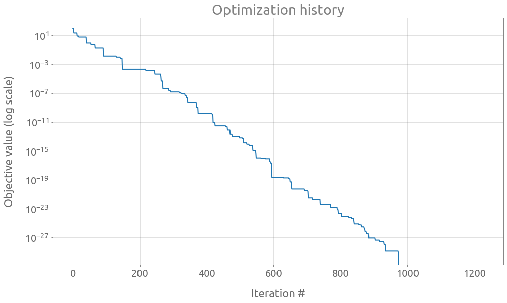
One way to reach another minimum is to change the random seed:

# Optuna' Sampler
sampler = optuna.samplers.CmaEsSampler(seed=1)
# Optuna' Study
study = optuna.create_study(sampler=sampler)

# reset the EarlyStoppingExceeded class
EarlyStoppingExceeded.early_stop = OPTUNA_EARLY_STOPING
EarlyStoppingExceeded.early_stop_count = 0
EarlyStoppingExceeded.best_score = None

try:
    study.optimize(
        objective, n_trials=50000, timeout=600, callbacks=[early_stopping_opt]
    )
except EarlyStoppingExceeded:
    print(f"EarlyStopping Exceeded: No new best scores on iters {OPTUNA_EARLY_STOPING}")

EarlyStopping Exceeded: No new best scores on iters 250

study.best_params

{'x': -2.805118086952745, 'y': 3.131312518250573}