Logistic regression with JAX
JAX is a Python package for automatic differentiation from Google Research. It is a really powerful and efficient library. JAX can automatically differentiate some Python code (supports the reverse- and forward-mode). It can also speed up the exection time by using the XLA (Accelerated Linear Algebra) compiler. JAX allows your code to run efficiently on CPUs, GPUs and TPUs. It is a library mainly used for machine learning. We refer to the The Autodiff Cookbook [2] for a very good introduction to JAX.
Photo credit: Papou Moustache
In this post we are going to simply use JAX’ grad function (back-propagation) to minimize the cost function of Logistic regression. In case you don’t know, Logistic regression is a supervised learning algorithm, for classification.
Here are the steps of this post:
- load a toy dataset
- briefly describe Logistic regression
- derive the formulae for the Logistic regression cost
- create a cost gradient function with JAX
- learn the Logistic regression weights with two gradient-based minimization methods: Gradient descent and BFGS
Imports
We import JAX’ NumPy instead of the regular one.
import warnings

warnings.filterwarnings("ignore", category=UserWarning)

import jax.numpy as jnp
from jax import grad
import matplotlib.pyplot as plt
from scipy.optimize import minimize
from sklearn.datasets import load_breast_cancer
from sklearn.preprocessing import StandardScaler
from sklearn.model_selection import train_test_split
from sklearn.metrics import classification_report

FS = (8, 4)  # figure size
RS = 124  # random seed
Load, split and scale the dataset
The breast cancer dataset is a classic binary classification dataset that we load from scikit-learn. Dataset features:
| Classes | 2 |
| Samples per class | 212(0),357(1) |
| Samples total | 569 |
| Dimensionality | 30 |
| Features | real, positive |
X, y = load_breast_cancer(return_X_y=True)
n_feat = X.shape[1]
X_train, X_test, y_train, y_test = train_test_split(
    X, y, test_size=0.25, stratify=y, random_state=RS
)
scaler = StandardScaler()
scaler.fit(X_train)
X_train_s = scaler.transform(X_train)
X_test_s = scaler.transform(X_test)
Logistic regression
Here we are going to look at the binary classification case, but it is straightforward to generalize the algorithm to multiclass classification using One-vs-Rest, or multinomial (Softmax) logistic regression.
Assume that we have $k$ predictors:
\[\left\{ X_i \right\}_{i=1}^{k} \in \mathbf{R}^k\]and a binary response variable:
\[Y \in \left\{ 0, 1 \right\}\]In the logistic regression algorithm, the relationship between the predictors and the $logit$ of the probability of a positive outcome $Y=1$ is assumed to be linear:
\begin{equation} logit( P(Y=1 | \textbf{w} ) ) = c + \sum_{i=1}^k w_i X_i \tag{1} \end{equation}
where
\[\left\{ w_i \right\}_{i=1}^{k} \in \mathbf{R}^k\]are the linear weights and $c \in \mathbf{R}$ the intercept. Now what is the $logit$ function? It is the log of odds:
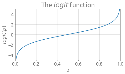
\begin{equation} logit( p ) = \ln \left( \frac{p}{1-p} \right) \tag{2} \end{equation}
We see that the $logit$ function is a way to map a probability value from $(0, 1)$ to $\mathbf{R}$:
eps = 1e-3
p = jnp.linspace(eps, 1 - eps, 200)
_, ax = plt.subplots(figsize=FS)
plt.plot(p, jnp.log(p / (1 - p)))
ax.grid()
_ = ax.set(xlabel="p", ylabel="$logit(p)$", title="The $logit$ function")
_ = ax.set_xlim(0, 1)
_ = ax.set_ylim(-5, 5)
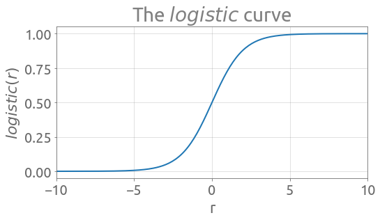
The inverse of the $logit$ is the $logistic$ curve (also called sigmoid function), which we are going to note $\sigma$:
\begin{equation} \sigma (r) = \frac{1}{1 + e^{-r}} \tag{3} \end{equation}
Here is the implementation of the $logistic$ curve:
def logistic(r):
    return 1 / (1 + jnp.exp(-r))


b = 10
r = jnp.linspace(-b, b, 200)
_, ax = plt.subplots(figsize=FS)
plt.plot(r, logistic(r))
ax.grid()
_ = ax.set(xlabel="r", ylabel="$logistic(r)$", title="The $logistic$ curve")
_ = ax.set_xlim(-b, b)
If we denote by $\textbf{w} = \left[c \; w_1 \; … \; w_k \right]^T$ the weight vector, $\textbf{x} = \left[ 1 \; x_1 \; … \;x_k \right]^T$ the observed values of the predictors, and $y$ the associated class value, we have:
\begin{equation} logit( P(y=1 | \textbf{w} ) ) = \textbf{w}^T \textbf{x} \tag{4} \end{equation}
And thus:
\begin{equation} P(y=1 | \textbf{w} )= \sigma(\textbf{w}^T \textbf{x} ) \equiv \sigma_{\textbf{w}} (\textbf{x}) \tag{5} \end{equation}
For a given set of weights $\textbf{w}$, the probability of a positive outcome is $\sigma_{\textbf{w}} (\textbf{x})$ that we implement in the following predict function:
def predict(c, w, X):
    return logistic(jnp.dot(X, w) + c)
This probability can be turned into a predicted class label $\hat{y}$ using a threshold value:
\[\hat{y} = 1 \; \text{if} \; \sigma_{\textbf{w}} (\textbf{x}) \geq 0.5, \; 0 \; \text{otherwise} \tag{6}\]The cost funtion
Now we assume that we have $n$ observations and that they are independently Bernoulli distributed:
\[\left\{ \left( \textbf{x}^{(1)}, y^{(1)} \right), \left( \textbf{x}^{(2)}, y^{(2)} \right), ..., \left( \textbf{x}^{(n)}, y^{(n)} \right) \right\}\]The likelihood that we would like to maximize given the samples is the following one:
\begin{equation} L(\textbf{w}) = \prod_{i=1}^n P( y^{(i)} | \textbf{x}^{(i)}; \textbf{w}) = \prod_{i=1}^n \sigma_{\textbf{w}} \left(\textbf{x}^{(i)} \right)^{y^{(i)}} \left( 1- \sigma_{\textbf{w}} \left(\textbf{x}^{(i)} \right)\right)^{1-y^{(i)}} \tag{7} \end{equation}
For some reasons related to numerical stability, we prefer to deal with a scaled log-likelihood. Also, we take the negative, in order to get a minimization problem:
\begin{equation} J(\textbf{w}) = - \frac{1}{n} \sum_{i=1}^n \left[ y^{(i)} \log \left( \sigma_{\textbf{w}} \left(\textbf{x}^{(i)} \right) \right) + \left( 1-y^{(i)} \right) \log \left( 1- \sigma_{\textbf{w}} \left(\textbf{x}^{(i)} \right)\right) \right] \tag{8} \end{equation}
A great feature of this cost function is that it is differentiable and convex. A gradient-based algorithm should find the global minimum. Now let’s also introduce some $l_2$-regularization in order to improve the model:
\begin{equation} J_r(\textbf{w}) = J(\textbf{w}) + \frac{\lambda}{2} \textbf{w}^T \textbf{w} \tag{9} \end{equation}
with $\lambda \geq 0$. As written by Sebastian Raschka in [1]:
Regularization is a very useful method to handle collinearity (high correlation among features), filter out noise from data, and eventually prevent overfitting.
Here is the cost function from Eq.$(9)$, $J_r(\textbf{w})$:
def cost(c, w, X, y, eps=1e-14, lmbd=0.1):
    n = y.size
    p = predict(c, w, X)
    p = jnp.clip(p, eps, 1 - eps)  # bound the probabilities within (0,1) to avoid ln(0)
    return -jnp.sum(y * jnp.log(p) + (1 - y) * jnp.log(1 - p)) / n + 0.5 * lmbd * (
        jnp.dot(w, w) + c * c
    )
We can now evaluate the cost function for some given values of $\textbf{w}$:
c_0 = 1.0
w_0 = 1.0e-5 * jnp.ones(n_feat)
print(cost(c_0, w_0, X_train_s, y_train))
0.7271773
We can also perform a prediction on the test dataset, but using weights that are very far from optimal:
y_pred_proba = predict(c_0, w_0, X_test_s)
y_pred_proba[:5]
DeviceArray([0.7310729 , 0.7310529 , 0.73104334, 0.7310562 , 0.7310334 ], dtype=float32)
and convert the resulting probabilities to predicted class labels:
y_pred = jnp.array(y_pred_proba)
y_pred = jnp.where(y_pred < 0.5, y_pred, 1.0)
y_pred = jnp.where(y_pred >= 0.5, y_pred, 0.0)
y_pred[:5]
DeviceArray([1., 1., 1., 1., 1.], dtype=float32)
This prediction is not so good, as expected:
print(classification_report(y_test, y_pred))
              precision    recall  f1-score   support

           0       0.00      0.00      0.00        57
           1       0.60      1.00      0.75        86

    accuracy                           0.60       143
   macro avg       0.30      0.50      0.38       143
weighted avg       0.36      0.60      0.45       143
Learning the weights
So we need to minimize $J_r(\textbf{w})$. For that we are going to apply two different algorithms:
- Gradient descent
- BFGS
They both use gradient $\nabla_{\textbf{w}} J_r(\textbf{w})$.
Compute the gradient
We could definitely compute the gradient of this Logistic regression cost function analytically. However we won’t, because we are are lazy and want JAX to do it for us! However, we can say that JAX would be more relevant if applied to a very complex function for which an analytical derivative is very hard or impossible to compute, such as the cost function of a deep neural network for example.
So let’s differentiate this cost function with respect to the first and second positional arguments using JAX’ grad function. Here is the derivative with respect to the intercept $c$:
print(grad(cost, argnums=0)(c_0, w_0, X_train_s, y_train))
0.19490835
And here is the gradient with respect to the other weights $\left[w_1 \; … \; w_k \right]^T$:
print(grad(cost, argnums=1)(c_0, w_0, X_train_s, y_train))
[ 0.3548751   0.19858086  0.36013606  0.3432787   0.16739811  0.28374672
  0.3358652   0.37103614  0.16127907 -0.01301905  0.2716888  -0.02297289
  0.26268682  0.25861    -0.05540825  0.14209975  0.12593843  0.19165947
 -0.02546574  0.03931254  0.37642777  0.21218807  0.37781695  0.3545265
  0.18594304  0.28257003  0.31803223  0.37415543  0.19396219  0.15303871]
Note that the grad function returns a function.
Gradient descent
From wikipedia:
Gradient descent is a first-order iterative optimization algorithm for finding a local minimum of a differentiable function.
The Gradient descent algorithm is very basic, here is an outline:
$w=w_0$
for $i = 1, …, n_{iter}$:
$ \hspace{1cm} w \leftarrow w - \eta \nabla_{\textbf{w}} J_r(\textbf{w})$
with $\eta >0$ small enough (that we can see as the learning rate).
And here is an implementation in which we added a stopping criterion (exits the loop if it stagnates during 20 iterations):
%%time
n_iter = 1000
eta = 5e-2
tol = 1e-6
w = w_0
c = c_0
new_cost = float(cost(c, w, X_train_s, y_train))
cost_hist = [new_cost]
for i in range(n_iter):
    c_current = c
    c -= eta * grad(cost, argnums=0)(c_current, w, X_train_s, y_train)
    w -= eta * grad(cost, argnums=1)(c_current, w, X_train_s, y_train)
    new_cost = float(cost(c, w, X_train_s, y_train))
    cost_hist.append(new_cost)
    if (i > 20) and (i % 10 == 0):
        if jnp.abs(cost_hist[-1] - cost_hist[-20]) < tol:
            print(f"Exited loop at iteration {i}")
            break
Exited loop at iteration 680
CPU times: user 20.6 s, sys: 1.8 s, total: 22.4 s
Wall time: 18.5 s
Let’s plot the convergence history:
_, ax = plt.subplots(figsize=FS)
plt.semilogy(cost_hist)
ax.grid()
_ = ax.set(xlabel="Iteration", ylabel="Cost value", title="Convergence history")
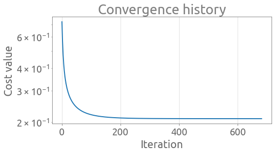
We can evaluate the trained model on the test set and check that the result is OK:
y_pred_proba = predict(c, w, X_test_s)
y_pred = jnp.array(y_pred_proba)
y_pred = jnp.where(y_pred < 0.5, y_pred, 1.0)
y_pred = jnp.where(y_pred >= 0.5, y_pred, 0.0)
print(classification_report(y_test, y_pred))
              precision    recall  f1-score   support

           0       0.96      0.96      0.96        57
           1       0.98      0.98      0.98        86

    accuracy                           0.97       143
   macro avg       0.97      0.97      0.97       143
weighted avg       0.97      0.97      0.97       143
BFGS
From wikipedia:
The BFGS method belongs to quasi-Newton methods, a class of hill-climbing optimization techniques that seek a stationary point of a (preferably twice continuously differentiable) function.
We are going to use SciPy’s implementation and give the grad function from JAX as an input parameter. Let’s first define the objective function with a single input vector (instead of c and w)
def fun(coefs):
    c = coefs[0]
    w = coefs[1:]
    return cost(c, w, X_train_s, y_train).astype(float)
%%time
res = minimize(
    fun,
    jnp.hstack([c_0, w_0]),
    method="BFGS",
    jac=grad(fun),
    options={"gtol": 1e-4, "disp": True},
)
Optimization terminated successfully.
         Current function value: 0.209017
         Iterations: 15
         Function evaluations: 16
         Gradient evaluations: 16
CPU times: user 480 ms, sys: 39.9 ms, total: 520 ms
Wall time: 445 ms
Much faster with a similar result!
c = res.x[0]
w = res.x[1:]
y_pred_proba = predict(c, w, X_test_s)
y_pred = jnp.array(y_pred_proba)
y_pred = jnp.where(y_pred < 0.5, y_pred, 1.0)
y_pred = jnp.where(y_pred >= 0.5, y_pred, 0.0)
print(classification_report(y_test, y_pred))
              precision    recall  f1-score   support

           0       0.96      0.96      0.96        57
           1       0.98      0.98      0.98        86

    accuracy                           0.97       143
   macro avg       0.97      0.97      0.97       143
weighted avg       0.97      0.97      0.97       143
Well we hardly scratched the surface of what can be done with JAX, but at least we presented a little example.
References:
Both references are really great ressources:
[1] S. Raschka and V. Mirjalili, Python Machine Learning, 2nd edition, Packt Publishing Ltd, Packt Publishing Ltd, 2017.
[2] alexbw@, mattjj@, The Autodiff Cookbook