Benford's law and the population of french cities

In this Python notebook, we are going to look at Benford’s law, which predicts the leading digit distribution, when dealing with some real-world collections of numbers. This distribution usually occurs when the numbers are rather smoothly distributed over several orders of magnitute. This can be observed with population data, file size data, stock prices, river lengths, …

We are going to check this law with a dataset of the population of all french cities (actually all settlements), as a simple experiment.

Finally, we will look at the generalized version of this first-digit law : the significant-digit law, which also predicts the occurence of other significant digits.

Imports

from zipfile import ZipFile

import requests
import numpy as np
import pandas as pd
import matplotlib.pyplot as plt

FS = (16, 9)  # figure size

Benford’s law

Here is the definition from wikipedia :

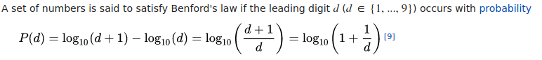
This was first discovered by Canadian-American astronomer Simon Newcomb in 1881, when he

noticed that in logarithm tables the earlier pages (that started with 1) were much more worn than the other pages.

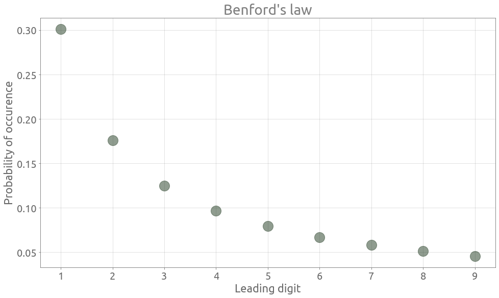
Let’s have a look at this distribution :

benford = pd.DataFrame(
    data={
        "proba": [np.log10(1 + 1 / d) for d in range(1, 10)],
        "leading_digit": range(1, 10),
    }
).set_index("leading_digit")
ax = benford.plot(
    legend=False, grid=True, alpha=0.5, figsize=FS, rot=0, style="o", ms=20
)
_ = ax.set(
    title="Benford's law", 
    xlabel="Leading digit", 
    ylabel="Probability of occurence"
)

Now let’s check our population data.

Population of french cities

Data from 2017 can be found here, from the website of the french institute of statistics and economic studies (INSEE). The chosen archive has several CSV files dealing with various administrative levels. We are going to use the commune level. Regarding population, communes are the same thing as cities when they have more than 2000 inhabitants, except for the 3 largest cities: Paris, Marseille and Lyon, where a commune corresponds to an “arrondissement”, which is some kind of district (e.g. twenty arrondissements in Paris). Below 2000 inhabitants, they correspond to villages. The data covers mainland France as well as overseas departments and regions.

Let’s start by downloading and extracting the data :

url = "https://www.insee.fr/fr/statistiques/fichier/4265429/ensemble.zip"
r = requests.get(url, allow_redirects=True)
file_name = "ensemble.zip"
_ = open(file_name, "wb").write(r.content)
with ZipFile(file_name, "r") as zip:
    zip.extractall()
!ls *.csv

Arrondissements.csv		     meta_arrondissements.csv
Cantons_et_metropoles.csv	     meta_associe.csv
Collectivites_d_outre_mer.csv	     meta_cantons.csv
Communes.csv			     meta_com.csv
Communes_associees_ou_deleguees.csv  meta_communes.csv
Departements.csv		     meta_departements.csv
Fractions_cantonales.csv	     meta_fractions.csv
Regions.csv			     meta_regions.csv

The communes.csv file has 5 columns and 34995 rows :

df = pd.read_csv("Communes.csv", sep=";")
df.head(2)

	DEPCOM	COM	PMUN	PCAP	PTOT
0	01001	L' Abergement-Clémenciat	776	18	794
1	01002	L' Abergement-de-Varey	248	1	249

DEPCOM is some kind of ID code
COM is the commune name
PTOT is the total population
We are only interested in the PTOT column.

df = df[df.PTOT > 0].copy(deep=True)

number_of_records = len(df)
min_value = df.PTOT.min()
max_value = df.PTOT.max()
orders_of_magnitude = int(np.log10(max_value)) - int(np.log10(min_value))
print(f"number_of_records : {number_of_records}")
print(f"min value : {min_value}")
print(f"max_value : {max_value}")
print(f"orders of magnitude : {orders_of_magnitude}")

number_of_records : 34989
min value : 1
max_value : 484809
orders of magnitude : 5

Now we store the leading digit and compute the probability of occurence :

df["leading_digit"] = df.PTOT.map(lambda x: int(str(x)[0]))
ld_occ_proba = df.leading_digit.value_counts() / len(df)

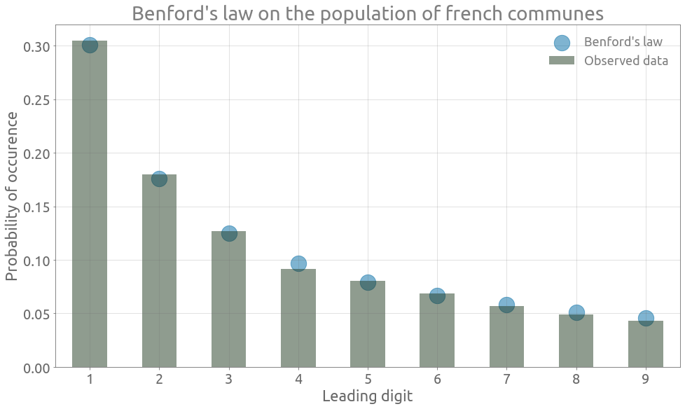
We can observe that the data follows Benford’s law pretty well :

ax = ld_occ_proba.plot.bar(figsize=FS, alpha=0.5, label="Observed data")
ax = benford.reset_index(drop=False).plot.scatter(
    x="leading_digit",
    y="proba",
    marker="o",
    s=500,
    ax=ax,
    alpha=0.5,
    label="Benford's law",
)
ax.grid()
_ = ax.set(
    title="Benford's law on the population of french communes",
    xlabel="Leading digit",
    ylabel="Probability of occurence",
)
_ = ax.set_ylim(
    0,
)
_ = ax.legend()

Quick explanation

First we can observe that the values of Benford’s distribution corresponds to the spacing in a log scale bar :

_ = plt.subplots(1, 1, figsize=FS)
ymin, ymax = -1, 1
xs = [0] + list(benford.proba.cumsum().values)
for x in xs:
    plt.vlines(x, ymin, ymax)
xs_h = [0.5 * (xs[i] + xs[i + 1]) for i in range(len(xs) - 1)]
for i, x in enumerate(xs_h):
    plt.text(x - 0.01, 0, str(i + 1), fontsize=25)

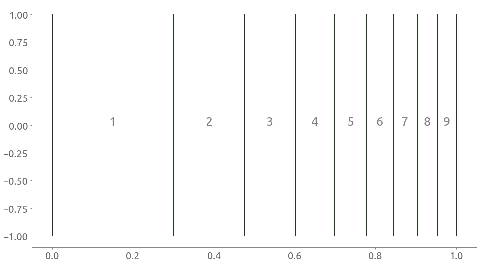
So if numbers are uniformly distributed in the log space over one order of magnitude, the probability that they start with the digit $i$ is actually equal to the width of the $i$-th column above : \begin{equation} P(D_1= d) = log_{10}(d+1) - log_{10}(d) = log_{10} \left( 1 + \frac{1}{d} \right) \end{equation}

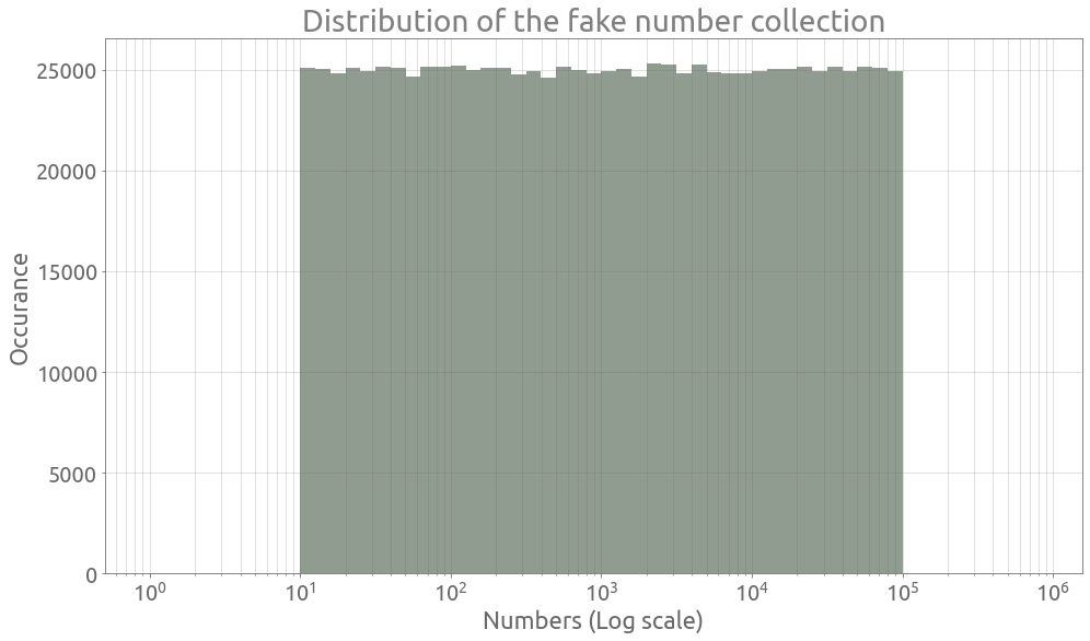
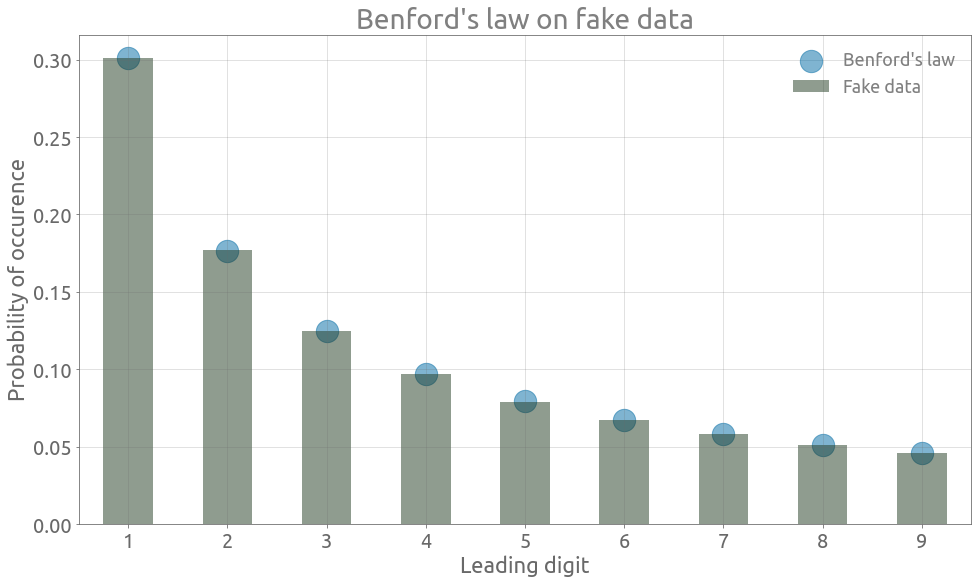
Let’s generate some fake numbers uniformly in the log space, across several orders of magnitude, and check that they perfectly follow Benford’s law :

n = 1_000_000
l, u = 1, 5
fake = pd.DataFrame(data={"gen": 10 ** (l + (u - l) * np.random.rand(n))})

coef = 10
bins = 10 ** (np.arange(0, 6 * coef) / coef)
plt.figure(figsize=FS)
plt.xscale("log")
plt.grid(True, which="both", ls="-")
_ = plt.hist(fake.gen.values, bins=bins, alpha=0.5)
_ = plt.xlabel("Numbers (Log scale)")
_ = plt.ylabel("Occurance")
_ = plt.title("Distribution of the fake number collection")

fake["leading_digit"] = fake.gen.map(lambda x: int(str(x)[0]))
fake_ld_occ_proba = fake.leading_digit.value_counts() / len(fake)

ax = fake_ld_occ_proba.plot.bar(figsize=FS, alpha=0.5, label="Fake data")
ax = benford.reset_index(drop=False).plot.scatter(
    x="leading_digit",
    y="proba",
    marker="o",
    s=500,
    ax=ax,
    alpha=0.5,
    label="Benford's law",
)
ax.grid()
_ = ax.set(
    title="Benford's law on fake data",
    xlabel="Leading digit",
    ylabel="Probability of occurence",
)
_ = ax.set_ylim(
    0,
)
_ = ax.legend()

If we look at the population’s distribution in the log space, we can see that it is rather spread out, across several orders of magnitude.

coef = 10
bins = 10 ** (np.arange(0, 6 * coef) / coef)
plt.figure(figsize=FS)
plt.xscale("log")
plt.grid(True, which="both", ls="-")
n, bins, patches = plt.hist(df.PTOT.values, bins=bins, alpha=0.5)
_ = plt.xlabel("Population (Log scale)")
_ = plt.ylabel("Occurance")
_ = plt.title("Distribution of the communes' population")

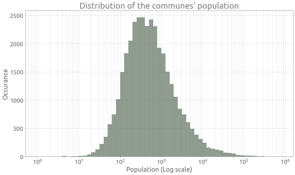
So even if it is not uniform in the log space, it is smooth and wide enough to approximately follow Bendford’s law. As explained in wikipedia:

Benford’s law can be seen in the larger area covered by red (first digit one) compared to blue (first digit 8) shading.

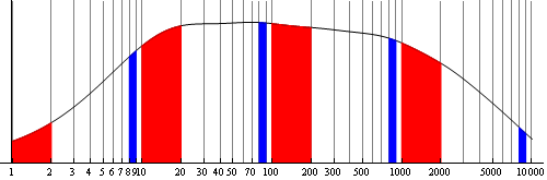
For each order of magnitude, the width corresponding to the leading digit 1 is almost 6 times larger than the one corresponding to the leading digit 8. So overall, the cumulative area under the distribution curve corresponding to the leading digit 1 is also about 6 times larger than the one corresponding to the leading digit 8.

Now, an interesting thing is that it Bendford’s law can be easily generalized to every significant digit. Let’s apply the second-digit version of the law to the population dataset.

Second significant digit

Here is the generalization of Benford’s law, from Hill [1] :

\begin{equation} P(D_1 = d_1, … ,D_k = d_k) = log_{10} \left[ 1 + \left( \sum_{i=1}^k d_i 10^{k-i} \right)^{-1} \right], \; k \geq 1 \end{equation}

where $d_j$ is the $j$-th significant digit ($d_1 \in (1, …, 9)$ and $d_j \in (0, …, 9)$ for $j>1$).

So the distribution of the second digit is the following one :

\begin{equation} P(D_2 = d_2) = \sum_{d_1=1}^9 P(D_1 = d_1, D_2 = d_2) = \sum_{d_1=1}^9 log_{10} \left[ 1 + \frac{1}{10 \; d_1 + d_2} \right] \end{equation}

Let’s have a look at this second-digit distribution :

benford_2 = pd.DataFrame(data={"second_digit": range(10)}, index=range(10))

benford_2["proba"] = 0.0
for d1 in range(1, 10):
    benford_2.proba += np.log10(1 + 1 / (10 * d1 + benford_2.second_digit))

benford_2.set_index("second_digit", inplace=True)
ax = benford_2.plot(
    legend=False, grid=True, alpha=0.5, figsize=FS, rot=0, style="o", ms=20
)
_ = ax.set(
    title="Benford's law for the second significant digit",
    xlabel="Second significant digit",
    ylabel="Probability of occurence",
)

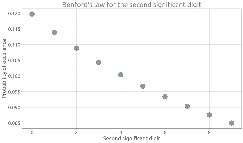
Although the second-digit distribution is not uniform, it is less uneven than the first-digit one.

Now we store the second digit and compute the probability of occurence :

df["second_digit"] = 0
df.loc[df.PTOT > 9, "second_digit"] = df[df.PTOT > 9].PTOT.map(lambda x: int(str(x)[1]))
sd_occ_pc = df.second_digit.value_counts() / len(df)

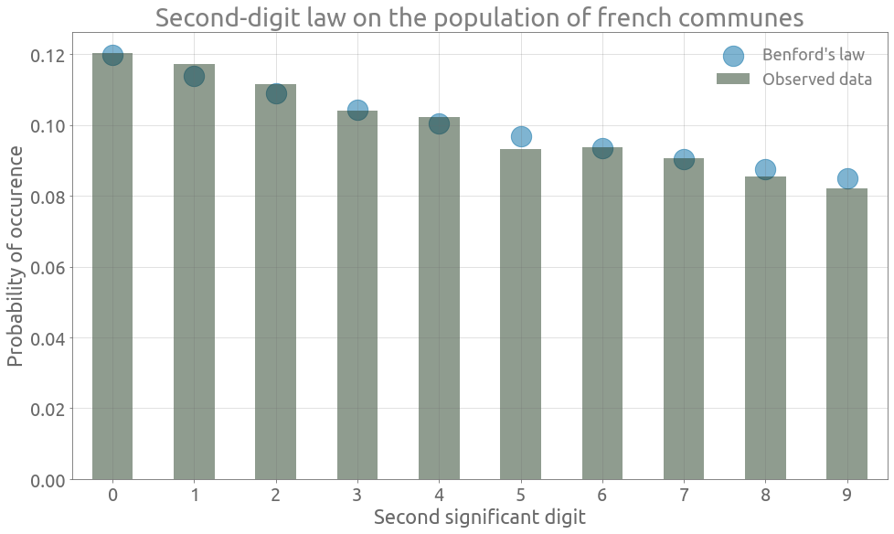
Again, we can observe that the data follows (the generalized) Benford’s law pretty well :

ax = sd_occ_pc.plot.bar(figsize=FS, alpha=0.5, label="Observed data")
ax = benford_2.reset_index(drop=False).plot.scatter(
    x="second_digit",
    y="proba",
    marker="o",
    s=500,
    ax=ax,
    alpha=0.5,
    label="Benford's law",
)
ax.grid()
_ = ax.set(
    title="Second-digit law on the population of french communes",
    xlabel="Second significant digit",
    ylabel="Probability of occurence",
)
_ = ax.set_ylim(
    0,
)
_ = ax.legend()

Reference

[1] Hill, Theodore P. A Statistical Derivation of the Significant-Digit Law. Statist. Sci. 10 (1995), no. 4, 354–363. doi:10.1214/ss/1177009869.