Saving a tf.keras model with data normalization

Training a DL model might take some time, and make use of some special hardware. So you may want to save the model for using it later, or on another computer.
In this short Python notebook, we are going to create a very simple tensorflow.keras model, train it, save it into a directory along with the training data scaling factors (standard scaling), and then load and call it.
The dataset is the breast cancer dataset from scikit-learn (binary classification). The point of this post is not the model but rather saving and loading the entire Keras model with the training dataset feature-wise mean and std.
Imports
import numpy as np
import pandas as pd
from sklearn import datasets
from sklearn.model_selection import train_test_split
from sklearn.metrics import accuracy_score
import tensorflow as tf

RS = 124  # random state
The package versions are the following ones :
CPython    3.7.8
tensorflow 2.3.0
pandas     0.25.3
sklearn    0.23.2
numpy      1.18.5
Data loading and train test split
X, y = datasets.load_breast_cancer(return_X_y=True)
X_train, X_test, y_train, y_test = train_test_split(
    X, y, test_size=0.3, stratify=y, random_state=RS
)
X.shape
(569, 30)
Data standardization with a Normalization layer
We are going to use a Normalization layer. As explained in the documentation :
This layer will coerce its inputs into a distribution centered around 0 with standard deviation 1. It accomplishes this by precomputing the mean and variance of the data, and calling (input-mean)/sqrt(var) at runtime.
layer = tf.keras.layers.experimental.preprocessing.Normalization()
layer.adapt(X_train)
Keras model
We use a very simple model :
tf.random.set_seed(RS)  # Sets the random seed

input_size = X_train.shape[1]

model = tf.keras.Sequential(
    [
        layer,
        tf.keras.layers.Dense(
            30,
            activation="sigmoid",
            input_shape=(input_size,),
        ),
        tf.keras.layers.Dense(
            16,
            activation="sigmoid",
        ),
        tf.keras.layers.Dense(1, activation="sigmoid"),
    ]
)
model.compile(
    optimizer=tf.keras.optimizers.Adam(
        learning_rate=0.001,
    ),
    loss="binary_crossentropy",
    metrics=["accuracy"],
)
print(model.summary())
Model: "sequential_1"
_________________________________________________________________
Layer (type)                 Output Shape              Param #
=================================================================
normalization_1 (Normalizati (None, 30)                61
_________________________________________________________________
dense_3 (Dense)              (None, 30)                930
_________________________________________________________________
dense_4 (Dense)              (None, 16)                496
_________________________________________________________________
dense_5 (Dense)              (None, 1)                 17
=================================================================
Total params: 1,504
Trainable params: 1,443
Non-trainable params: 61
_________________________________________________________________
None
Training
history = model.fit(
    X_train,
    y_train,
    epochs=40,
    batch_size=32,
    verbose=0,
)
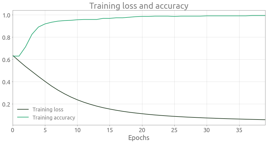
ax = pd.DataFrame(data=history.history).plot(figsize=(15, 7))
ax.grid()
_ = ax.set(title="Training loss and accuracy", xlabel="Epochs")
_ = ax.legend(["Training loss", "Trainig accuracy"])

If we evaluate the model on the test set, we get an accuracy of 0.9708:
results = model.evaluate(X_test, y_test, verbose=1)
6/6 [==============================] - 0s 12ms/step - loss: 0.1053 - accuracy: 0.9708
OK, now that the model is trained, let’s save it!
Save the whole model
It is possible to partially save the model. However, here we are going to save the entire model with model.save(). As described in the documentation :
You can save an entire model to a single artifact. It will include :
- The model’s architecture/config
- The model’s weight values (which were learned during training)
- The model’s compilation information (if compile()) was called
- The optimizer and its state, if any (this enables you to restart training where you left)
Note that since we only load the model for inference in the later part of the post, we do not actually need the two last points.
MODEL_PATH = "./tf_model"
model.save(MODEL_PATH)
INFO:tensorflow:Assets written to: ./tf_model/assets
!tree {MODEL_PATH}
./tf_model
├── assets
├── saved_model.pb
└── variables
    ├── variables.data-00000-of-00001
    └── variables.index

2 directories, 3 files
The model architecture, and training configuration (including the optimizer, losses, and metrics) are stored in
saved_model.pb. The weights are saved in thevariables/directory.
Loading the model
model = tf.keras.models.load_model(MODEL_PATH)
Calling the model
Note that the normalization layer is automatically used in the inference.
y_pred_proba = model.predict(X_test, verbose=0)[:, 0]
y_pred_proba[:4]
array([0.02198085, 0.37227017, 0.0198662 , 0.99156594], dtype=float32)
y_pred = np.where(y_pred_proba < 0.5, 0, 1)
y_pred[:4]
array([0, 0, 0, 1])
print(f"accuracy score : {accuracy_score(y_test, y_pred):5.4f}")
accuracy score : 0.9708