Goldbach's Comet with Numba and Datashader

Updated Jul 29, 2021

This Python notebook is about computing and plotting Goldbach function. It requires some basic mathematical knowledge, nothing fancy! The main point is to perfom some computations with Numba and some efficient plotting with Datashader.

Here is the definition of the Goldbach function from wikipedia:

The function $g ( E )$ is defined for all even integers $E > 2$ to be the number of different ways in which E can be expressed as the sum of two primes. For example, $g ( 22 ) = 3$ since 22 can be expressed as the sum of two primes in three different ways ( 22 = 11 + 11 = 5 + 17 = 3 + 19).

The different prime pairs $(p_1, p_2)$ that sum to an even integer $E=p_1+p_2$ are called Goldbach partitions.

Note that for Goldbach’s conjecture to be false, there must be $g(E) = 0$ somewhere for $E > 2$. Anyway, here are the steps used in this notebook to compute Goldbach function. Given a maximum positive integer $n$:

• For each natural number smaller or equal to $n$, build a quick way to check if it is a prime or not, and also list the corresponding primes. In order to do that, we are going to use the sieve of Eratosthenes.
• for each even number $E$ smaller or equal to $n$, compute $g(E)$ by counting the number of cases where $E-p$ is prime for all primes $p$ not larger than $E/2$.

If $E-p$ is prime for a given prime $p \leq E/2$ then $(p, E-p)$ is indeed a partition of $E$. We count all the partitions for $E$ by looping over all primes $p \leq E/2$, .

Imports

from typing import Tuple

import numpy as np
import pandas as pd
import primesieve
from numba import jit, njit, prange
import matplotlib.pyplot as plt
import perfplot
import datashader as ds
from datashader import transfer_functions as tf
from colorcet import palette

FS_R = (20, 10)  # rectangular figure size
FS_S = (10, 10)  # square figure size

Package versions:

    Python    : 3.9.6
    pandas    : 1.3.0
    datashader: 0.13.0
    primesieve: 2.3.0
    matplotlib: 3.4.2
    numpy     : 1.21.1
    colorcet  : 2.0.6
    perfplot  : 0.9.6
    numba     : 0.53.1

Sieve of Eratosthenes

Simple implementation with Numba

This code is inspired from wikipedia and geeksforgeeks. It flags all primes not greater than $n$. The algorithm includes a common optimization, which is to start enumerating the multiples of each prime $p$ from $p^2$.

@jit(nopython=True)
def generate_is_prime_vector(n: int) -> np.ndarray:

    # initialize all entries as True, except 0 and 1
    is_prime_vec = np.ones(n + 1, dtype=np.bool_)
    is_prime_vec[0:2] = False

    # loop on prime numbers
    p = 2
    while p * p <= n:
        if is_prime_vec[p] == True:
            # Update all multiples of p, starting from p * p
            for i in range(p * p, n + 1, p):
                is_prime_vec[i] = False
        p += 1

    return is_prime_vec

Let’s run it with a small value of n:

n = 11
is_prime_vec = generate_is_prime_vector(n)
is_prime_vec

array([False, False,  True,  True, False,  True, False,  True, False,
       False, False,  True])

We can get the list of primes from is_prime_vec using np.flatnonzero:

primes = np.flatnonzero(is_prime_vec).astype(np.uint64)
primes

array([ 2,  3,  5,  7, 11], dtype=uint64)

Using primesieve

As an alternate way, these two arrays, primes and is_prime_vec, can be computed using the optimized C/C++ primesieve library:

primes = np.array(primesieve.primes(n))
primes

array([ 2,  3,  5,  7, 11], dtype=uint64)

is_prime_vec = np.zeros(n + 1, dtype=np.bool_)
is_prime_vec[primes] = True
is_prime_vec

array([False, False,  True,  True, False,  True, False,  True, False,
       False, False,  True])

Value check

As a sanity check, we compare the prime lists obtained with the different methods for a larger value of n:

def generate_primes_simple(n: int) -> Tuple[np.ndarray, np.ndarray]:
    is_prime_vec = generate_is_prime_vector(n)
    primes = np.flatnonzero(is_prime_vec).astype(np.uint64)
    return primes, is_prime_vec

def generate_primes_primesieve(n: int) -> Tuple[np.ndarray, np.ndarray]:
    primes = np.array(primesieve.primes(n))
    is_prime_vec = np.zeros(n + 1, dtype=np.bool_)
    is_prime_vec[primes] = True
    return primes, is_prime_vec

%%time
n = 1_000_000
primes_1, is_prime_vec_1 = generate_primes_simple(n)
primes_2, is_prime_vec_2 = generate_primes_primesieve(n)
np.testing.assert_array_equal(primes_1, primes_2)
np.testing.assert_array_equal(is_prime_vec_1, is_prime_vec_2)

CPU times: user 36.5 ms, sys: 15 µs, total: 36.5 ms
Wall time: 60.3 ms

Elapsed time

%%time
out = perfplot.bench(
    setup=lambda n: n,
    kernels=[
        lambda n: generate_primes_simple(n),
        lambda n: generate_primes_primesieve(n),    
    ],
    labels=["generate_primes_simple", "generate_primes_primesieve"],
    n_range=[10 ** k for k in range(1, 8)],
    equality_check=None
)
out

CPU times: user 7.2 s, sys: 281 ms, total: 7.48 s
Wall time: 7.3 s

┏━━━━━━━━━━┳━━━━━━━━━━━━━━━━━━━━━━━━┳━━━━━━━━━━━━━━━━━━━━━━━━━━━━┓
┃ n        ┃ generate_primes_simple ┃ generate_primes_primesieve ┃
┡━━━━━━━━━━╇━━━━━━━━━━━━━━━━━━━━━━━━╇━━━━━━━━━━━━━━━━━━━━━━━━━━━━┩
│ 10       │ 4.693000000000001e-06  │ 6.4000000000000006e-06     │
│ 100      │ 5.1700000000000005e-06 │ 6.233e-06                  │
│ 1000     │ 9.468e-06              │ 7.658e-06                  │
│ 10000    │ 3.2039e-05             │ 1.4255000000000002e-05     │
│ 100000   │ 0.000283582            │ 8.438300000000001e-05      │
│ 1000000  │ 0.004541556            │ 0.000679709                │
│ 10000000 │ 0.07260718000000001    │ 0.008423457                │
└──────────┴────────────────────────┴────────────────────────────┘

ms = 10
fig = plt.figure(figsize=FS_S)
ax = fig.add_subplot(1, 1, 1)
plt.loglog(
    out.n_range,
    1.0e-8 * out.n_range * np.log(np.log(out.n_range)),
    "-",
    label="$O(n \, log \, log \, n)$",
)
plt.loglog(out.n_range, out.timings_s[0], "v-", ms=ms, label="generate_primes_simple")
plt.loglog(
    out.n_range, out.timings_s[1], "^-", ms=ms, label="generate_primes_primesieve"
)
plt.legend()
plt.grid(True)
_ = ax.set_ylabel("Runtime [s]")
_ = ax.set_xlabel("n")
_ = ax.set_title("Timings of the generate_primes functions")

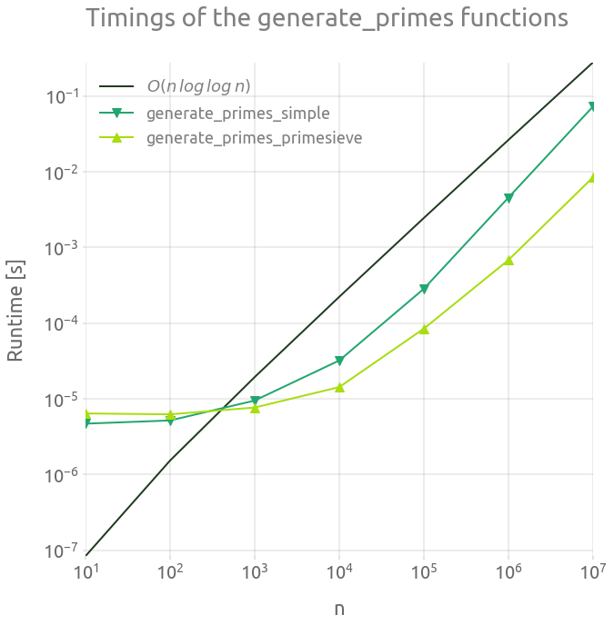
The run time of both of these generate_primes functions is very small compared to the rest of the Goldbach function evaluation. Anyway, the primesieve version is way more efficient, so we are going to stick with it in the following. Note that is it is supposed to have a run time complexity of $0(n \, log \, log \, n)$ operations.

The timings of the generate_primes_simple function in pure Python (without Numba) is not shown. It is usually slower by a factor 10 or 100 (100 is more likely than 10 for this kind of CPU bound function).

Find the number of prime pairs for a given even number E

Now we show how $g(E)$ can be computed for a given value of $E$. We are going to compare 3 different implementations with Numba.

Three different implementations

In the fist version, compute_g_1, we loop over all natural numbers $2 \leq i \leq E/2$. If $i$ and $E-i$ are primes, then $(i, E-1)$ is a partition. The function compute_g_1 takes the is_prime_vec boolean vector as argument, but not the primes array.

@jit(nopython=True)
def compute_g_1(is_prime_vec: np.ndarray, E: int) -> int:

    assert E < len(is_prime_vec)
    assert E % 2 == 0
    E_half = int(0.5 * E)

    # initialization
    i = 2  # loop counter (we know that 0 and 1 are not primes)
    count = 0  # number of prime pairs

    # we loop over all the prime numbers smaller than or equal to half of num
    while i <= E_half:
        if is_prime_vec[i] and is_prime_vec[E - i]:
            count += 1
        i += 1

    return count

In the second version, we loop on primes $p$ instead on integers, with a while loop:

• If $E-p$ is a prime, $(p, E-P)$ is a partition.
• If $p > E/2$, we exit the loop.

The function compute_g_2 takes both is_prime_vec and primes as arguments:

@jit(nopython=True)
def compute_g_2(is_prime_vec: np.ndarray, primes: np.ndarray, E: int) -> int:

    assert E < len(is_prime_vec)
    assert E % 2 == 0
    E_half = int(0.5 * E)

    # initialization
    count = 0  # number of prime pairs

    # we loop over all the prime numbers smaller than or equal to half of num
    i = 0
    p = primes[i]
    while p <= E_half:

        if is_prime_vec[E - p]:
            count += 1
        i += 1
        p = primes[i]

    return count

The third function compute_g_3 is similar to the previous one, but uses a for loop instead of while. The upper bound of the for loop is computed using np.searchsorted, since primes are sorted within the primes vector.

@jit(nopython=True)
def compute_g_3(is_prime_vec: np.ndarray, primes: np.ndarray, E: int) -> int:

    assert E < len(is_prime_vec)
    assert E % 2 == 0
    E_half = int(0.5 * E)

    # initialization
    count = 0  # number of prime pairs

    # we loop over all the prime numbers smaller than or equal to half of num
    i_max = np.searchsorted(primes, E_half, side="right")
    for i in range(i_max):
        p = primes[i]
        if is_prime_vec[E - p]:
            count += 1

    return count

Value check

%%time
E = 22
assert E % 2 == 0
assert E > 0
n = 100
primes, is_prime_vec = generate_primes_primesieve(n)
print(compute_g_1(is_prime_vec, E))
print(compute_g_2(is_prime_vec, primes, E))
print(compute_g_3(is_prime_vec, primes, E))

3
3
3
CPU times: user 1.04 s, sys: 3.89 ms, total: 1.04 s
Wall time: 1.12 s

Elapsed time

%%time
out = perfplot.bench(
    setup=lambda n: generate_primes_primesieve(n),
    kernels=[
        lambda x: compute_g_1(x[1], len(x[1])-1),
        lambda x: compute_g_2(x[1], x[0], len(x[1])-1),    
        lambda x: compute_g_3(x[1], x[0], len(x[1])-1),
    ],
    labels=["compute_g_1", "compute_g_2", "compute_g_3"],
    n_range=[10 ** k for k in range(3, 8)],
    equality_check=None
)
out

CPU times: user 11.3 s, sys: 111 ms, total: 11.4 s
Wall time: 11.9 s

┏━━━━━━━━━━┳━━━━━━━━━━━━━━━━━━━━━━━┳━━━━━━━━━━━━━━━━━━━━━━━━┳━━━━━━━━━━━━━━━━━━━━━━━┓
┃ n        ┃ compute_g_1           ┃ compute_g_2            ┃ compute_g_3           ┃
┡━━━━━━━━━━╇━━━━━━━━━━━━━━━━━━━━━━━╇━━━━━━━━━━━━━━━━━━━━━━━━╇━━━━━━━━━━━━━━━━━━━━━━━┩
│ 1000     │ 1.072e-06             │ 9.660000000000002e-07  │ 1.057e-06             │
│ 10000    │ 1.147e-05             │ 2.2370000000000004e-06 │ 1.825e-06             │
│ 100000   │ 8.608e-05             │ 1.0703e-05             │ 7.805e-06             │
│ 1000000  │ 0.0009804660000000001 │ 8.4447e-05             │ 5.1739e-05            │
│ 10000000 │ 0.00576324            │ 0.000573377            │ 0.0005268870000000001 │
└──────────┴───────────────────────┴────────────────────────┴───────────────────────┘

ms = 10
fig = plt.figure(figsize=FS_S)
ax = fig.add_subplot(1, 1, 1)
plt.loglog(
    out.n_range,
    1.0e-9 * out.n_range,
    "-",
    label="$O(n)$",
)
plt.loglog(out.n_range, out.timings_s[0], "v-", ms=ms, label="compute_g_1")
plt.loglog(out.n_range, out.timings_s[1], "^-", ms=ms, label="compute_g_2")
plt.loglog(out.n_range, out.timings_s[2], "^-", ms=ms, label="compute_g_3")
plt.legend()
plt.grid(True)
_ = ax.set_ylabel("Runtime [s]")
_ = ax.set_xlabel("n")
_ = ax.set_title("Timings of the compute_g functions")

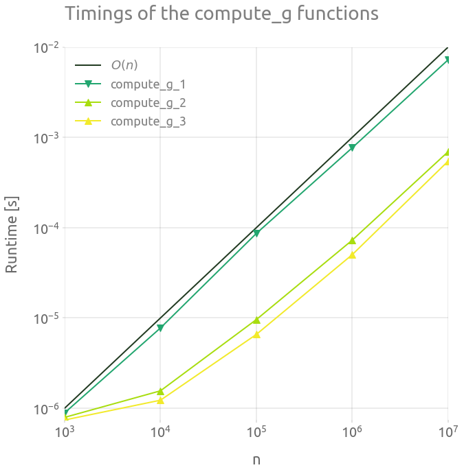
The compute_g_3 is the most efficient of the three variations. Let’s use this approach to compute many value of $g(E)$.

The algorithms’ complexity is $O(n)$, because we basically loop over an array proportional to $n$ to perform a $O(1)$ operation.

Loop over all even numbers E smaller or equal to n

Now we simply loop over all even natural numbers $E \leq n$ to compute all respective values of $g(E)$. Note that in the following compute_g_vector_seq function, the outer loop has a step size of 1, in order to later use Numba prange, which only supports this unit step size. This means that we loop on contiguous integer values of $E/2$ instead of even values of $E$. Also, we compute is_prime_vec and primes only once and use it for all the evaluations of $g(E)$.

n is calculted from the length of is_prime_vec. In the arguments, we assume that primes is corresponding to the primes of is_prime_vec.

Sequential loop

@jit(nopython=True)
def compute_g_vector_seq(is_prime_vec: np.ndarray, primes: np.ndarray) -> np.ndarray:

    n_max = len(is_prime_vec) - 1
    n_max_half = int(0.5 * n_max) + 1

    g_vec = np.empty(n_max_half, dtype=np.uint)

    for E_half in range(n_max_half):
        count = 0
        E = 2 * E_half
        i_max = np.searchsorted(primes, E_half, side="right")
        for i in range(i_max):
            p = primes[i]
            if is_prime_vec[E - p]:
                count += 1
        g_vec[E_half] = np.uint(count)

    return g_vec

The $i$-th value of g_vec correponds to $g(2 \, i)$ with $i \geq 0 $:

i	E	g_vec[i]
0	0	0
1	2	0
2	4	1
3	6	1
4	8	1
5	10	2

and so on…

Parallel loop

We are now going to parallelize compute_g_vector_seq by using the Numba njit decorator and prange on the outer explicit loop. The vector g_vec is shared across threads but each thread is only writing into its own partition.

@njit(parallel=True)
def compute_g_vector_par(is_prime_vec: np.ndarray, primes: np.ndarray) -> np.ndarray:

    n_max = len(is_prime_vec) - 1
    n_max_half = int(0.5 * n_max) + 1

    g_vec = np.empty(n_max_half, dtype=np.uint)

    for E_half in prange(n_max_half):
        count = 0
        E = 2 * E_half
        i_max = np.searchsorted(primes, E_half, side="right")
        for i in range(i_max):
            p = primes[i]
            if is_prime_vec[E - p]:
                count += 1

        g_vec[E_half] = np.uint(count)

    return g_vec

We can check $g$ at least for some for some small values of $E$:

n = 56
primes, is_prime_vec = generate_primes_primesieve(n)
g_vec_1 = compute_g_vector_seq(is_prime_vec, primes)
g_vec_2 = compute_g_vector_par(is_prime_vec, primes)
g_vec_ref = [0, 0, 1, 1, 1, 2, 1, 2, 2, 2, 2, 3, 3, 3, 2, 3, 2, 4, 4, 2, 3, 4, 
    3, 4, 5, 4, 3, 5, 3]
np.testing.assert_array_equal(g_vec_1, g_vec_ref)
np.testing.assert_array_equal(g_vec_2, g_vec_ref)

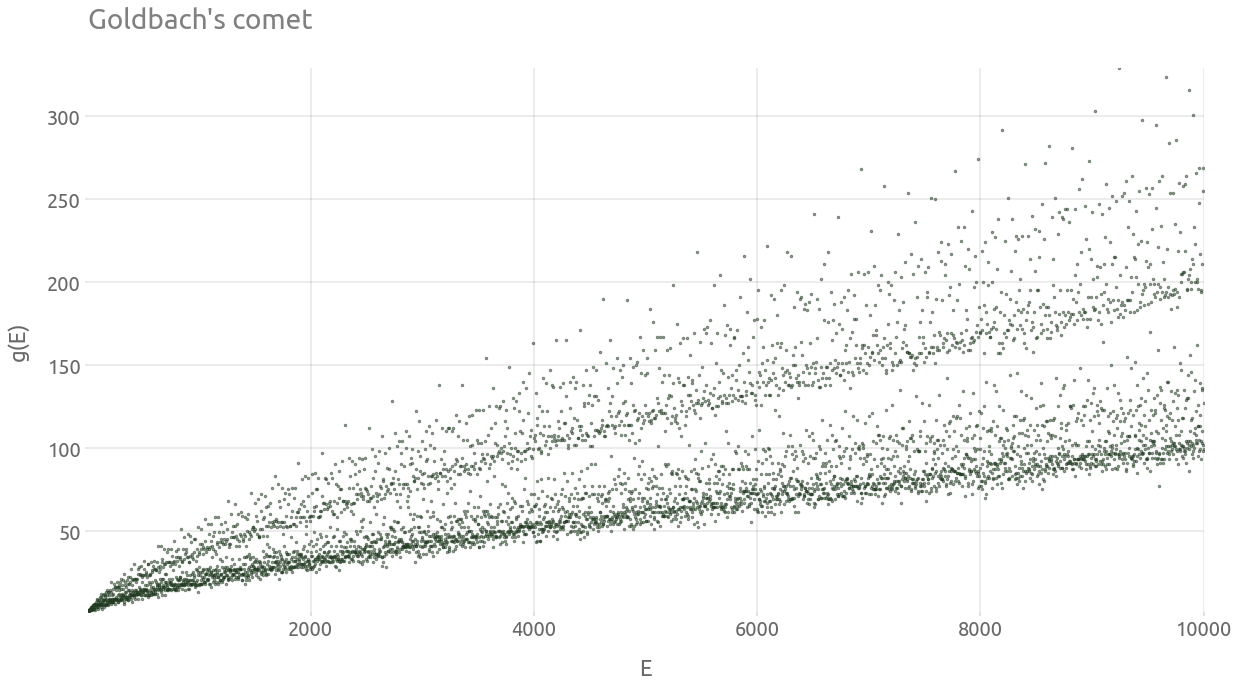
First plot of the comet

%%time
n = 10_000
primes, is_prime_vec = generate_primes_primesieve(n)
g_vec = compute_g_vector_par(is_prime_vec, primes)
g_df = pd.DataFrame(data={"g": g_vec}, index=2 * np.arange(len(g_vec)))
g_df = g_df[g_df.index > 2]  # The function g(E) is defined for all even integers E>2
g_df.head(2)

CPU times: user 19.1 ms, sys: 0 ns, total: 19.1 ms
Wall time: 4.36 ms

	g
4	1
6	1

ax = g_df.plot(style=".", ms=5, alpha=0.5, legend=False, figsize=FS_R)
_ = ax.set(
    title="Goldbach's comet",
    xlabel="E",
    ylabel="g(E)",
)
ax.autoscale(enable=True, axis="x", tight=True)
ax.grid(True)

Elapsed time

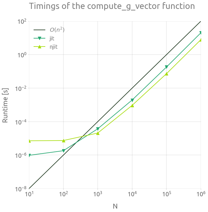
Now we compare the running time of the sequential and parallel versions of compute_g_vector. The code is running on a laptop with 8 cores (Intel(R) i7-7700HQ CPU @ 2.80GHz).

%%time
out = perfplot.bench(
    setup=lambda n: generate_primes_primesieve(n),
    kernels=[
        lambda x: compute_g_vector_seq(x[1], x[0]),
        lambda x: compute_g_vector_par(x[1], x[0]),
    ],
    labels=["jit", "njit"],
    n_range=[10 ** k for k in range(1, 7)],
)
out

CPU times: user 1min 18s, sys: 265 ms, total: 1min 19s
Wall time: 35.6 s

┏━━━━━━━━━┳━━━━━━━━━━━━━━━━━━━━━━━━┳━━━━━━━━━━━━━━━━━━━━━━━┓
┃ n       ┃ jit                    ┃ njit                  ┃
┡━━━━━━━━━╇━━━━━━━━━━━━━━━━━━━━━━━━╇━━━━━━━━━━━━━━━━━━━━━━━┩
│ 10      │ 9.740000000000001e-07  │ 7.213e-06             │
│ 100     │ 1.8400000000000002e-06 │ 7.474000000000001e-06 │
│ 1000    │ 3.7302e-05             │ 2.0854e-05            │
│ 10000   │ 0.001960103            │ 0.0009358410000000001 │
│ 100000  │ 0.182704941            │ 0.07333213200000001   │
│ 1000000 │ 20.137010665000002     │ 7.841122203           │
└─────────┴────────────────────────┴───────────────────────┘

Basically, running the parallel version on 8 cores divides the running time by a factor 2 to 3.

ms = 10
fig = plt.figure(figsize=FS_S)
ax = fig.add_subplot(1, 1, 1)
plt.loglog(
    out.n_range,
    1.0e-10 * np.power(out.n_range, 2),
    "-",
    label="$O(n^2)$",
)
plt.loglog(out.n_range, out.timings_s[0], "v-", ms=ms, label="jit")
plt.loglog(out.n_range, out.timings_s[1], "^-", ms=ms, label="njit")
plt.legend()
plt.grid("on")
_ = ax.set_ylabel("Runtime [s]")
_ = ax.set_xlabel("N")
_ = ax.set_title("Timings of the compute_g_vector function")

If we run the parallel version with $n=1e6$, we might estimate if the running time with a larger value of $n$ is affordable.

%%time
n = 1_000_000
primes, is_prime_vec = generate_primes_primesieve(n)
g_vec = compute_g_vector_par(is_prime_vec, primes)

CPU times: user 26.5 s, sys: 23.5 ms, total: 26.6 s
Wall time: 6.28 s

So computing $g$ with $n = 5e6$ should take one or two minutes on my laptop with compute_g_vector_par… Let’s do that next.

Compute a larger vector of g values

%%time
n = 5_000_000
primes, is_prime_vec = generate_primes_primesieve(n)
g_vec = compute_g_vector_par(is_prime_vec, primes)

CPU times: user 8min 33s, sys: 6.11 ms, total: 8min 33s
Wall time: 1min 37s

g_df = pd.DataFrame(data={"E": 2 * np.arange(len(g_vec)), "g": g_vec})
g_df = g_df[g_df.E > 2]  # The function g(E) is defined for all even integers E>2

Plotting g with Datashader

cmap = palette["dimgray"]
bg_col = "white"
height = 800
width = int(np.round(1.6 * height))

%%time
cvs = ds.Canvas(plot_width=width, plot_height=height)
agg = cvs.points(g_df, "E", "g")
img = tf.shade(agg, cmap=cmap)
img = tf.set_background(img, bg_col)
img

CPU times: user 1.1 s, sys: 16 ms, total: 1.12 s
Wall time: 1.11 s

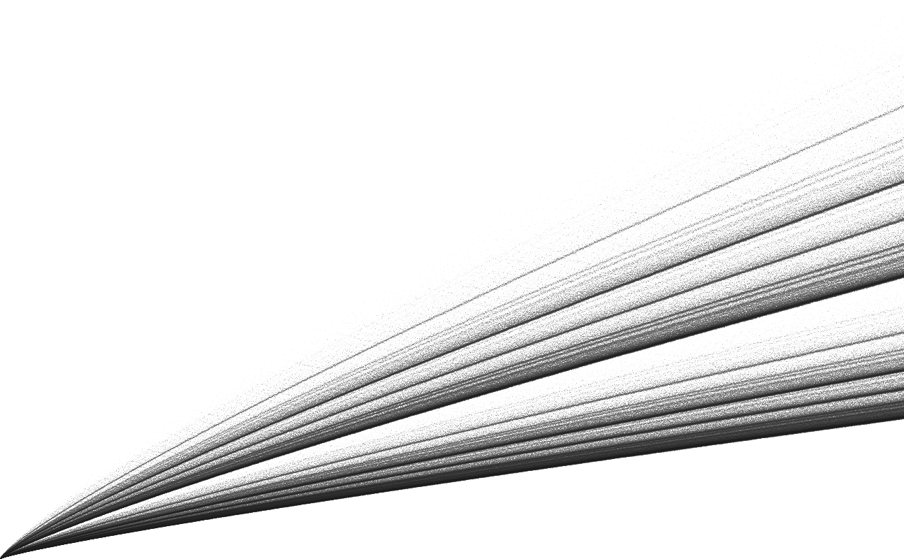
We can clearly observe some dense lines in this “comet tail”. In order to visualize this vertical distribution of prime pairs count, we are are going to normalize $g$. As explained on the wikipedia page:

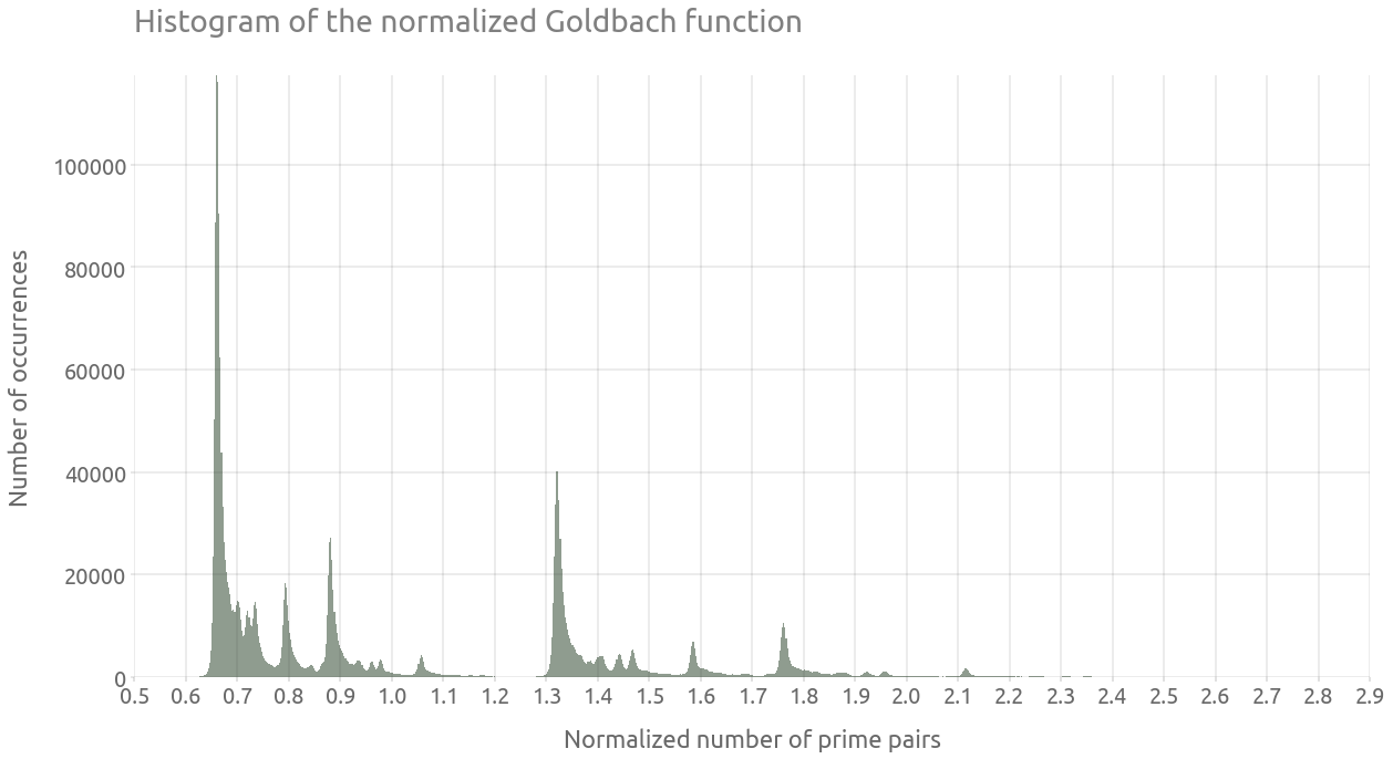
An illuminating way of presenting the comet data is as a histogram. The function g(E) can be normalized by dividing by the locally averaged value of g, gav, taken over perhaps 1000 neighboring values of the even number E. The histogram can then be accumulated over a range of up to about 10% either side of a central E.

%%time
g_df["g_av"] = g_df["g"].rolling(window=1000, center=True).mean()
g_df["g_norm"] = g_df["g"] / g_df["g_av"]

CPU times: user 128 ms, sys: 23.9 ms, total: 152 ms
Wall time: 153 ms

%%time
cvs = ds.Canvas(plot_width=width, plot_height=height)
agg = cvs.points(g_df, "E", "g_norm")
img = tf.shade(agg, cmap=cmap)
img = tf.set_background(img, bg_col)
img

CPU times: user 885 ms, sys: 12 ms, total: 897 ms
Wall time: 908 ms

We can now proceed to plot the histogram of the comet data, which will lead to some kind of cross section of the above plot:

ax = g_df["g_norm"].hist(bins=1000, alpha=0.5, figsize=(20, 10))
ax.grid(True)
_ = ax.set(
    title="Histogram of the normalized Goldbach function",
    xlabel="Normalized number of prime pairs",
    ylabel="Number of occurrences",
)
_ = plt.xticks(np.arange(0.5, 3.0, 0.1))

The Hardy-Littlewood estimate

As described on the wikipedia page for Goldbach’s comet, the number of Goldbach partitions can be estimated using the following formulae from Hardy and Littlewood (1922):

\[\frac{g(E)}{g_{av}} = \Pi_2 \prod \frac{p-1}{p-2}\]

where the product is taken over all primes p that are factors of $E/2$, $\Pi_2$ being the twin primes constant:

\[\Pi_2 = \prod_{p \geq 3} \left( 1 - \frac{1}{(1-p)^2} \right)\]

%%time
n = 100_000_000
primes = np.array(primesieve.primes(n))

# twin primes constant
Pi2 = np.prod(1.0 - 1.0 / np.power(1.0 - primes[1:], 2))
Pi2

CPU times: user 318 ms, sys: 76 ms, total: 394 ms
Wall time: 405 ms

0.6601618161644595

So let’s compute this estimate of the normalized Goldbach function with Numba njit:

@njit(parallel=True)
def compute_g_hl_vector_par(primes: np.ndarray, n_max: int, Pi2: float) -> np.ndarray:

    n_max_half = int(0.5 * n_max) + 1

    g_hl_vec = np.empty(n_max_half, dtype=np.float64)

    for E_half in prange(n_max_half):
        i_max = np.searchsorted(primes, E_half, side="right")
        prod = 1.0
        for i in range(1, i_max):
            p = primes[i]
            if E_half % p == 0:
                prod *= (p - 1.0) / (p - 2.0)

        g_hl_vec[E_half] = np.float64(prod)
    g_hl_vec *= Pi2

    return g_hl_vec

%%time
n = 1_000_000
g_hl_vec = compute_g_hl_vector_par(np.array(primesieve.primes(n)), n, Pi2)

CPU times: user 1min 17s, sys: 83 ms, total: 1min 17s
Wall time: 18.1 s

Plotting the estimate with Datashader

g_hl_df = pd.DataFrame(data={"E": 2 * np.arange(len(g_hl_vec)), "g_norm": g_hl_vec})

%%time
cvs = ds.Canvas(plot_width=width, plot_height=height)
agg = cvs.points(g_hl_df, "E", "g_norm")
img = tf.shade(agg, cmap=cmap)
img = tf.set_background(img, bg_col)
img

CPU times: user 106 ms, sys: 16 ms, total: 122 ms
Wall time: 117 ms

The vertical distribution of the dense lines seems to be similar to the one from the normalized Goldbach function. This can be checked by computing and plotting both kernel density estimates.

Kernel density estimates

%%time
ax = g_df["g_norm"].plot.density(alpha=0.5, figsize=FS_R, label='Golbach function')
ax = g_hl_df.g_norm.plot.density(alpha=0.5, ax=ax, label='Hardy-Littlewood estimate')
ax.grid(True)
_ = ax.set(
    title="KDEs of the normalized Goldbach function and its Hardy-Littlewood estimate",
    xlabel="Normalized number of prime pairs",
    ylabel="Density",
)
_ = ax.legend()
_ = plt.xticks(np.arange(0.5, 3.0, 0.1))
_ = ax.set_xlim(0.5, 2.5)

CPU times: user 1min 6s, sys: 792 ms, total: 1min 6s
Wall time: 1min 5s

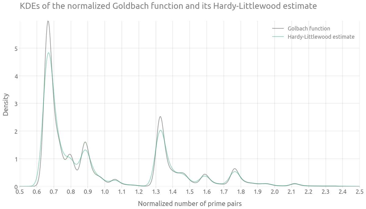
Note that the Goldbach function is computed up to $n=5e6$, against $n=1e6$ for the estimate, which might explain some of the differences between the densities. However, we can clearly observe that the peaks are located at the same places.

Prime E/2 values only

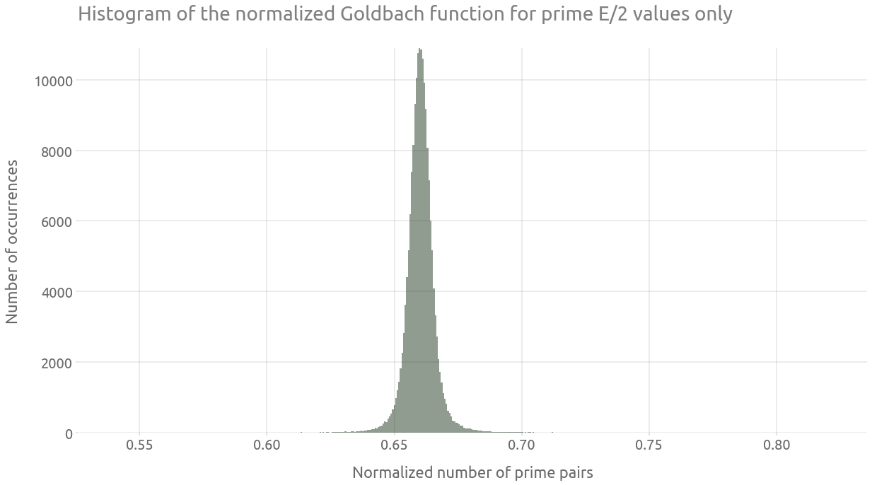
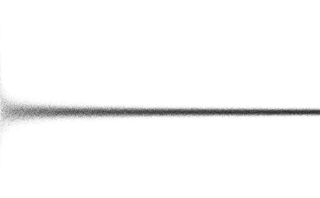
Finally, we are going to isolate a part of the most dense line from the comet tail (for a normalized number of prime pairs around 0.66). As explained in wikipedia:

Of particular interest is the peak formed by selecting only values of E/2 that are prime. […] The peak is very close to a Gaussian form.

g_df["E_half"] = (0.5 * g_df["E"]).astype(int)
g_df_primes = g_df[g_df["E_half"].isin(primes)]

%%time
cvs = ds.Canvas(plot_width=width, plot_height=height)
agg = cvs.points(g_df_primes, "E", "g_norm")
img = tf.shade(agg, cmap=cmap)
img = tf.set_background(img, bg_col)
img

CPU times: user 97.9 ms, sys: 3.98 ms, total: 102 ms
Wall time: 99.7 ms

ax = g_df_primes["g_norm"].hist(bins=500, alpha=0.5, figsize=FS_R)
ax.grid(True)
_ = ax.set(
    title="Histogram of the normalized Goldbach function for prime E/2 values only",
    xlabel="Normalized number of prime pairs",
    ylabel="Number of occurrences",
)