Spatial Join with GeoPandas (and GEOS)
Updated Sep 13, 2021
![]()
The purpose of this post is to perform an “efficient” spatial join in Python. What is a spatial join? Here is the definition from wiki.gis.com:
A Spatial join is a GIS operation that affixes data from one feature layer’s attribute table to another from a spatial perspective.
For example, in the following, we are going to perform a spatial join between a point layer and a polygon layer. One of the attributes of the polygon layer is a string code that we want to attach to the points located within each polygon.
Warning: the time measurements given in the following correspond to different Jupyter sessions with various other jobs running alongside, so they would vary if run again. They are only presented to provide an order of magnitude.
The Datasets
Point layer
The point dataset deals with real estate price. Its called DVF and is provided by the french open data. Here is a description from data.gouv.fr:
The “Requests for real estate values” database, or DVF, lists all the sales of real estate made over the last five years, in mainland France and in the overseas departments and territories - except in Mayotte and Alsace-Moselle. The goods concerned can be built (apartment and house) or not built (land lot, fields).
The locations of most of these real estate transfers have been geocoded, so they exhibit some longitude and latitude attributes. The data can be downloaded from here as yearly CSVs. For a given year, different files correspond to different levels of administrative divisions (communes, departements):
Index of /geo-dvf/latest/csv/2020/
../
communes/                                          01-Jun-2021 15:30                   -
departements/                                      01-Jun-2021 15:30                   -
full.csv.gz                                        01-Jun-2021 12:48            71045047
However, here we are going to use the “full” data files corresponding to the whole territory: full2016.csv.gz, full2017.csv.gz, …, full2020.csv.gz. Although data is only available for the last five years, we also included 2 previously collected files: full2014.csv.gz and full2015.csv.gz, for a total 7 years time span. This results in a dataframe with 19 895 888 rows (note that a property transfer can hold several distinct rows).
The csv files have been previously loaded with Pandas, concatenated and saved as a Parquet file. Here is the snippet used (dfv_fps is a list with the gzipped CSV file paths):
df = pd.DataFrame()
for fp in dfv_fps:
    df_tmp = pd.read_csv(fp, low_memory=False)
    df = pd.concat([df, df_tmp], axis=0)
df.date_mutation = pd.to_datetime(df.date_mutation)
df.sort_values(by="date_mutation", ascending=True, inplace=True)
df.reset_index(drop=True, inplace=True)
for col in ["lot1_numero", "lot2_numero", "lot3_numero", "lot4_numero", "lot5_numero"]:
    df[col] = df[col].astype(str)
df.to_parquet("dvf.parquet")
Polygon layer
For the polygon layer, we are going to use the IRIS zones. Here is a definition of these zones from INSEE (National Institute of Statistics and Economic Studies) website:
In order to prepare for the dissemination of the 1999 population census, INSEE developed a system for dividing the country into units of equal size, known as IRIS2000. In French, IRIS is an acronym of ‘aggregated units for statistical information’, and the 2000 refers to the target size of 2000 residents per basic unit. Since that time IRIS (the term which has replaced IRIS2000) has represented the fundamental unit for dissemination of infra-municipal data. These units must respect geographic and demographic criteria and have borders which are clearly identifiable and stable in the long term. Towns with more than 10,000 inhabitants, and a large proportion of towns with between 5,000 and 10,000 inhabitants, are divided into several IRIS units. This separation represents a division of the territory.
Data can be downloaded from here. We used the 2021 version from this ftp link:
ftp://Contours_IRIS_ext:ao6Phu5ohJ4jaeji@ftp3.ign.fr/CONTOURS-IRIS_2-1__SHP__FRA_2021-01-01.7z.
There are 48589 zones that forms a partition without overlap of mainland France and Corsica.
GeoPandas and PyGeos
Most of the treatments in the following are made with the great GeoPandas library, installed with conda:
conda install -c conda-forge geopandas
GeoPandas may use GEOS as an “booster”, using the PyGeos interface. Here is a presentation of PyGeos from its documentation:
PyGEOS is a C/Python library with vectorized geometry functions. The geometry operations are done in the open-source geometry library GEOS. PyGEOS wraps these operations in NumPy ufuncs providing a performance improvement when operating on arrays of geometries.
GEOS (Geometry Engine - Open Source) is a C++ port of the Java Topology Suite (JTS).
As explained in the GeoPandas documentation:
whether the speedups are used or not is determined by:
- If PyGEOS >= 0.8 is installed, it will be used by default (but installing GeoPandas will not yet automatically install PyGEOS as dependency, you need to do this manually).
- You can still toggle the use of PyGEOS when it is available, by […] setting an option: geopandas.options.use_pygeos = True/False. Note, although this variable can be set during an interactive session, it will only work if the GeoDataFrames you use are created (e.g. reading a file with read_file) after changing this value.
Here we installed pygeos version 0.10.2, which uses libgeos 3.9.1:
conda install pygeos --channel conda-forge
Imports
import contextily as ctx
from colorcet import palette
import datashader as ds
from datashader.mpl_ext import dsshow
import geopandas as gpd
from geopandas.tools import sjoin
import matplotlib.pyplot as plt
import pandas as pd
from pygeos import Geometry
import numpy as np
from shapely.geometry import Polygon, MultiPolygon
gpd.options.use_pygeos = True
Load/prepare the point data
In order to perform the spatial join, we only load 3 columns:
id_parcelleis a string identification for plots of land, that we are going to use later to join with the full dataset (attribute join).longitudeandlatitudeare the geographical coordinates (WGS 84 - EPSG:4326)
%%time
dvf_df = pd.read_parquet('dvf.parquet', columns=['id_parcelle', 'longitude', 'latitude'])
CPU times: user 6.03 s, sys: 1.43 s, total: 7.46 s
Wall time: 6.38 s
len(dvf_df)
19895888
dvf_df.dtypes
id_parcelle     object
longitude      float64
latitude       float64
dtype: object
Drop rows with missing coordinates:
dvf_df.dropna(subset=["latitude", "longitude"], how="any", inplace=True)
Only keep mainland France and Corsica:
bbox = (-5.06, 41.04, 9.91, 51.27)
dvf_df = dvf_df[
    (dvf_df.longitude > bbox[0])
    & (dvf_df.latitude > bbox[1])
    & (dvf_df.longitude < bbox[2])
    & (dvf_df.latitude < bbox[3])
]
len(dvf_df)
19118424
Plot the points
Let’s plot thes points with datashader using its native support for matplotlib. We start by loading the french border geometry as a geodataframe, after downloading the shapefile from the naturalearth website:
world = gpd.read_file("./admin_countries/ne_10m_admin_0_countries.shp")
france = world[(world.SOVEREIGNT == "France") & (world.TYPE == "Country")]["geometry"]
france.geometry.values[0] = MultiPolygon(
    [france.geometry.values[0][1], france.geometry.values[0][11]]  # extract mainland France and Corsica
)
We also make sure to use the same CRS (Coordinate Reference Systems) as for the points from the DVF dataset (EPSG:4326):
france.crs
<Geographic 2D CRS: EPSG:4326>
Name: WGS 84
Axis Info [ellipsoidal]:
- Lat[north]: Geodetic latitude (degree)
- Lon[east]: Geodetic longitude (degree)
Area of Use:
- name: World.
- bounds: (-180.0, -90.0, 180.0, 90.0)
Datum: World Geodetic System 1984 ensemble
- Ellipsoid: WGS 84
- Prime Meridian: Greenwich
%%time
cmap = palette["dimgray"][::-1]
fig, ax = plt.subplots(figsize=(15,15))
_ = dsshow(
    dvf_df,
    ds.Point("longitude", "latitude"),
    norm="eq_hist",
    cmap=cmap,
    ax=ax,
)
ax.grid(False)
ax.set_facecolor("white")
_ = ax.set(title="DVF points")
ax = france.plot(facecolor="none", edgecolor="black", ax=ax)
ax.set_axis_off()
CPU times: user 1.61 s, sys: 447 ms, total: 2.05 s
Wall time: 1.4 s
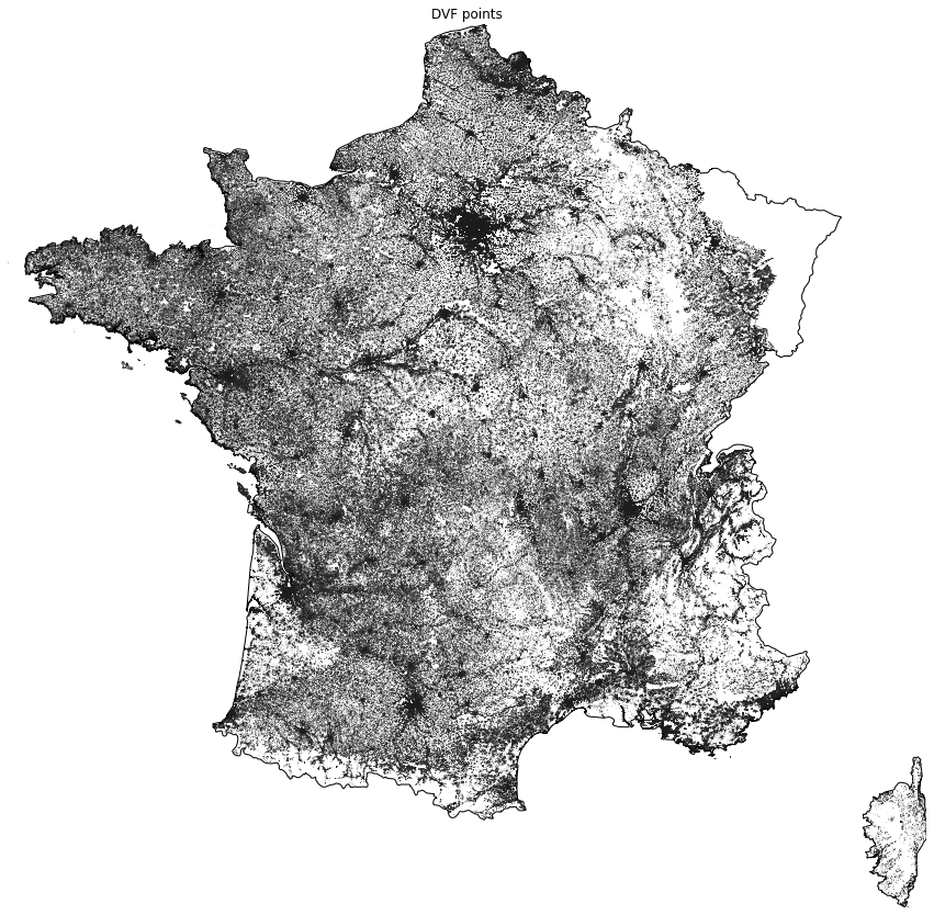
We can see that data for Alsace and Moselle are missing (top right) because they have a specific legal status.
We want to assign a single zone code (from a polygon) to each id_parcelle. So let’s keep a single geographical point per id_parcelle:
%%time
dvf_df.drop_duplicates(subset="id_parcelle", keep="first", inplace=True)
CPU times: user 8.85 s, sys: 557 ms, total: 9.41 s
Wall time: 9.44 s
len(dvf_df)
10256266
This reduces the size of the point dataset significantly! Let’s transform the dataframe into a geodataframe:
%%time
dvf_gdf = gpd.GeoDataFrame(
    dvf_df[['id_parcelle']], geometry=gpd.points_from_xy(dvf_df.longitude, dvf_df.latitude), crs="EPSG:4326")
del dvf_df
CPU times: user 1.86 s, sys: 649 ms, total: 2.51 s
Wall time: 1.98 s
This is where the GEOS library starts to make a significant difference regarding the elapsed time:
| With GEOS | Without GEOS |
|---|---|
| 1.98s | 4m 14s |
dvf_gdf.head(3)
| id_parcelle | geometry | |
|---|---|---|
| 0 | 16002000ZM0106 | POINT (0.20973 46.06524) |
| 1 | 830930000A2119 | POINT (5.71065 43.32764) |
| 2 | 830930000A2120 | POINT (5.71082 43.32771) |
dvf_gdf.isna().sum(axis=0)
id_parcelle    0
geometry       0
dtype: int64
Load/prepare the polygon data
%%time
iris_gdf = gpd.read_file(
    "CONTOURS-IRIS_2-1__SHP__FRA_2021-01-01/CONTOURS-IRIS/1_DONNEES_LIVRAISON_2021-06-00217/CONTOURS-IRIS_2-1_SHP_LAMB93_FXX-2021/CONTOURS-IRIS.shp"
)[['CODE_IRIS', 'geometry']]
iris_gdf.head(3)
CPU times: user 4.5 s, sys: 220 ms, total: 4.72 s
Wall time: 3.19 s
| CODE_IRIS | geometry | |
|---|---|---|
| 0 | 721910000 | POLYGON ((498083.500 6747517.400, 498128.000 6... |
| 1 | 772480000 | POLYGON ((685753.100 6868612.900, 685757.700 6... |
| 2 | 514260000 | POLYGON ((759067.200 6849592.700, 758778.600 6... |
There is no significant difference regarding the elapsed time with or without GEOS for this loading operation:
| With GEOS | Without GEOS |
|---|---|
| 3.19s | 3.94s |
len(iris_gdf)
48589
iris_gdf.geometry.map(lambda g: g.geom_type).value_counts()
Polygon         48333
MultiPolygon      256
Name: geometry, dtype: int64
iris_gdf.crs
<Projected CRS: EPSG:2154>
Name: RGF93 / Lambert-93
Axis Info [cartesian]:
- X[east]: Easting (metre)
- Y[north]: Northing (metre)
Area of Use:
- name: France - onshore and offshore, mainland and Corsica.
- bounds: (-9.86, 41.15, 10.38, 51.56)
Coordinate Operation:
- name: Lambert-93
- method: Lambert Conic Conformal (2SP)
Datum: Reseau Geodesique Francais 1993
- Ellipsoid: GRS 1980
- Prime Meridian: Greenwich
We need to use the same CRS between the point and polygon layers. So let’s convert the the polygon layer to EPSG4326:
%%time
iris_gdf = iris_gdf.to_crs("EPSG:4326")
CPU times: user 4.68 s, sys: 68.3 ms, total: 4.75 s
Wall time: 4.48 s
Again we observe an improvement with GEOS:
| With GEOS | Without GEOS |
|---|---|
| 4.48s | 10.6s |
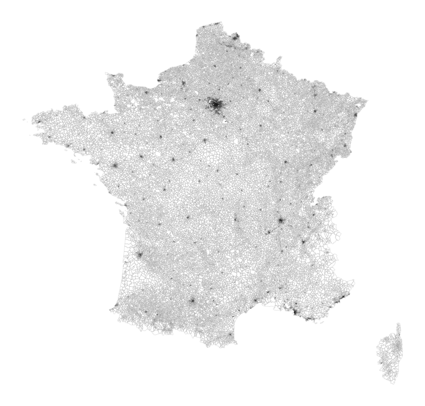
Plot the polygons
%%time
ax = iris_gdf.plot(facecolor="white", edgecolor="black", alpha=0.1, figsize=(15, 15))
ax.set_axis_off()
CPU times: user 17.8 s, sys: 228 ms, total: 18.1 s
Wall time: 18 s
Spatial indexing
In order to perform the spatial join between 10256266 points and 48589 Poygons/MultiPolygons, we need some spatial indexing. What is it? Here is a definition from ucgis.org:
A spatial index is a data structure that allows for accessing a spatial object efficiently. It is a common technique used by spatial databases. Without indexing, any search for a feature would require a “sequential scan” of every record in the database, resulting in much longer processing time. In a spatial index construction process, the minimum bounding rectangle serves as an object approximation. Various types of spatial indices across commercial and open-source databases yield measurable performance differences. Spatial indexing techniques are playing a central role in time-critical applications and the manipulation of spatial big data.
From GeoPandas documentation:
GeoPandas offers built-in support for spatial indexing using an R-Tree algorithm. Depending on the ability to import
pygeos,GeoPandaswill either usepygeos.STRtreeorrtree.index.Index.
So we won’t use the same piece of code with or without GEOS, but it will use some kind of R-trees in both cases. Here is the definition of R-trees from wikipedia:
R-trees are tree data structures used for spatial access methods, i.e., for indexing multi-dimensional information such as geographical coordinates, rectangles or polygons. The R-tree was proposed by Antonin Guttman in 1984 and has found significant use in both theoretical and applied contexts. A common real-world usage for an R-tree might be to store spatial objects such as restaurant locations or the polygons that typical maps are made of: streets, buildings, outlines of lakes, coastlines, etc. and then find answers quickly to queries such as “Find all museums within 2 km of my current location”, “retrieve all road segments within 2 km of my location” (to display them in a navigation system) or “find the nearest gas station” (although not taking roads into account).
Simple example of a R-tree for 2D rectangles from wikipedia:

The implementation in GEOS is a Sort-Tile-Recursive (STR) algorithm.
Let’s build the index.
dvf_gdf.has_sindex
False
%%time
dvf_gdf.sindex
CPU times: user 7.38 s, sys: 855 ms, total: 8.23 s
Wall time: 8.24 s

<geopandas.sindex.PyGEOSSTRTreeIndex at 0x7fa8b3e2c0a0>
| With GEOS | Without GEOS |
|---|---|
| 8.24s | 6min 15s |
With PyGeos we get a geopandas.sindex.PyGEOSSTRTreeIndex index object, otherwise we get a rtree.index.Index(bounds=[-5.059852, 41.363063, 9.557005, 51.082069], size=10256266).
Spatial join
Now we are going to perform a left join with a within operator (point-in-polygon). It seems that the intersects operator takes really more time in the current case.
%%time
dvf_gdf_sjoin = sjoin(
        dvf_gdf,
        iris_gdf[['CODE_IRIS', 'geometry']],
        how="left",
        op="within",
    )
dvf_gdf_sjoin.drop("index_right", axis=1, inplace=True)
CPU times: user 19.8 s, sys: 2.69 s, total: 22.5 s
Wall time: 17.7 s
| With GEOS | Without GEOS |
|---|---|
| 17.7s | 3min 1s |
dvf_gdf_sjoin.head(3)
| id_parcelle | geometry | CODE_IRIS | |
|---|---|---|---|
| 0 | 16002000ZM0106 | POINT (0.20973 46.06524) | 160020000 |
| 1 | 830930000A2119 | POINT (5.71065 43.32764) | 830930000 |
| 2 | 830930000A2120 | POINT (5.71082 43.32771) | 830930000 |
dvf_gdf_sjoin.isna().sum(axis=0)
id_parcelle       0
geometry          0
CODE_IRIS      2559
dtype: int64
So unfortunately 2559 points (over 10256266) did not match any zone.
Orphan points
Let’s isolate them:
%%time
orphans_gdf = dvf_gdf_sjoin[dvf_gdf_sjoin.CODE_IRIS.isna()].drop("CODE_IRIS", axis=1)
CPU times: user 833 ms, sys: 3.6 ms, total: 836 ms
Wall time: 842 ms
len(orphans_gdf)
2559
orphans_gdf.head(3)
| id_parcelle | geometry | |
|---|---|---|
| 2315 | 83019000BZ0030 | POINT (6.36461 43.12122) |
| 7559 | 11202000DX0019 | POINT (3.03670 42.86225) |
| 10843 | 34003000OK0003 | POINT (3.50888 43.27685) |
Plot the orphan points
ax = orphans_gdf.plot(figsize=(15, 15))
ax = france.plot(facecolor="none", edgecolor="black", ax=ax)
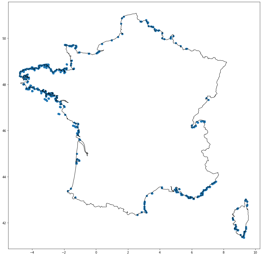
We can see that the orphans are all located at the outside border of the IRIS polygons. Let’s zoom in to see an area where a lot of points are orphans:
# Plouguerneau
bb = (-4.618113, 48.555804, -4.397013, 48.658866)
bb_polygon = Polygon([(bb[0], bb[1]), (bb[0], bb[3]), (bb[2], bb[3]), (bb[2], bb[1])])
bbox = gpd.GeoDataFrame(geometry=[bb_polygon], crs="EPSG:4326")
iris_zoom = gpd.overlay(iris_gdf, bbox, how="intersection")
orphans_zoom = gpd.overlay(orphans_gdf, bbox, how="intersection")
# Convert the data to Web Mercator to display some tiles
ax = orphans_zoom.to_crs("EPSG:3857").plot(color="r", markersize=25, figsize=(15, 15))
ax = iris_zoom.to_crs("EPSG:3857").plot(
    facecolor="none", edgecolor="k", linewidth=2, alpha=0.6, ax=ax
)
ctx.add_basemap(ax, source=ctx.providers.Stamen.Terrain)
ax.set_axis_off()
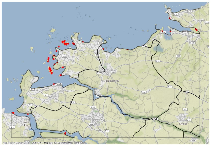
The poins may be orphans because they are located on a small island or because the IRIS contour is simplified and do not match exactly the actual land contour. So let’s perform a nearest query using the spatial index, in order to match each orphan point with the nearest IRIS polygon.
Nearest query
Although it is not mandatory here, we switch to a projected CRS before looking for the nearest zones. As explained here, this allows to minimize visual distortion in a particular region. Basically distances can be accurately measured in a projected CRS.
%%time
orphans_gpd = orphans_gdf.to_crs("EPSG:2154")  # RGF93 / Lambert-93 -- France
iris_gdf = iris_gdf.to_crs("EPSG:2154")
CPU times: user 2.79 s, sys: 103 ms, total: 2.89 s
Wall time: 2.9 s
| With GEOS | Without GEOS |
|---|---|
| 2.9s | 9.29 s |
iris_gdf.has_sindex
False
We see that the iris_gdf does not have an index, let’s do that with GEOS (very quick process):
iris_gdf.sindex
Note that the required indices are built automatically if needed when performing the spatial join. It is not required to call the index contructor by hand.
Now we create an array of pygeos.Geometry objects:
%%time
points_str = list(orphans_gdf.geometry.map(str).values)
points = np.vectorize(Geometry)(points_str)
points
CPU times: user 186 ms, sys: 560 µs, total: 186 ms
Wall time: 177 ms


array([<pygeos.Geometry POINT (6.36 43.1)>,
       <pygeos.Geometry POINT (3.04 42.9)>,
       <pygeos.Geometry POINT (3.51 43.3)>, ...,
       <pygeos.Geometry POINT (-3.15 47.3)>,
       <pygeos.Geometry POINT (-2.79 47.5)>,
       <pygeos.Geometry POINT (3.78 50.4)>], dtype=object)
Also, we need a function returning the nearest Polygon:
def find_nearest_idx(point):
    return iris_gdf.sindex.nearest(point)[1][0]
The following vectorization actually only works with GEOS. Otherwise we get the following error message:
TypeError: Bounds must be a sequence
%%time
indices = np.vectorize(find_nearest_idx)(points)
CPU times: user 459 ms, sys: 3.47 ms, total: 463 ms
Wall time: 459 ms
Here is for example the index of the nearest zone for the first orphan point:
indices[0]
18258
We can actually check is the distance method of GeoPandas returns the same index:
%%time
iris_gdf.distance(orphans_gdf.geometry.values[0]).sort_values().index[0]
CPU times: user 252 ms, sys: 0 ns, total: 252 ms
Wall time: 250 ms

18258
Attribute join
Now let’s put everything together:
orphans_gdf["CODE_IRIS"] = iris_gdf.iloc[indices].CODE_IRIS.values
orphans_gpd = orphans_gpd.to_crs("EPSG:4326")
dvf_gdf = pd.concat([dvf_gdf_sjoin.dropna(), orphans_gdf], axis=0)
dvf_gdf.isna().sum(axis=0)
id_parcelle    0
geometry       0
CODE_IRIS      0
dtype: int64
%%time
dvf_df = pd.read_parquet("dvf.parquet")
CPU times: user 57.8 s, sys: 9.53 s, total: 1min 7s
Wall time: 29.6 s
%%time
dvf_df = pd.merge(dvf_df, dvf_gdf[["id_parcelle", "CODE_IRIS"]], on="id_parcelle", how="left")
CPU times: user 1min 44s, sys: 28.3 s, total: 2min 12s
Wall time: 2min 12s
dvf_df.isna().sum(axis=0)
id_mutation                            0
date_mutation                          0
numero_disposition                     0
nature_mutation                        0
valeur_fonciere                   262966
adresse_numero                   8401364
adresse_suffixe                 19058836
adresse_nom_voie                  200632
adresse_code_voie                 185574
code_postal                       197452
code_commune                           0
nom_commune                            0
code_departement                       0
ancien_code_commune             19435502
ancien_nom_commune              19435502
id_parcelle                            0
ancien_id_parcelle              19781277
numero_volume                   19839247
lot1_numero                            0
lot1_surface_carrez             18251916
lot2_numero                            0
lot2_surface_carrez             19488477
lot3_numero                            0
lot3_surface_carrez             19855820
lot4_numero                            0
lot4_surface_carrez             19885521
lot5_numero                            0
lot5_surface_carrez             19891330
nombre_lots                            0
code_type_local                  9199398
type_local                       9199398
surface_reelle_bati             11885358
nombre_pieces_principales        9215887
code_nature_culture              6133795
nature_culture                   6133795
code_nature_culture_speciale    18972456
nature_culture_speciale         18972456
surface_terrain                  6134186
longitude                         610533
latitude                          610533
CODE_IRIS                         752239
dtype: int64
Remaining missing values for the CODE_IRIS column corresponds to rows with missing coordinates or locations outside mainland France or Corsica.
%%time
dvf_df.to_parquet("dvf_iris.parquet")