Applying a row-wise function to a Pandas dataframe
More than 3 years ago, we posted a comparative study about Looping over Pandas data using a CPU. Because a lot of things evolved since 2018, this post is kind of an update. For example Pandas tag version was 0.23.3 at that time, it is now 1.4.0. Also, we added some more options.
Here is a list of all the options tested in the following:
- Pandas built-in vectorization
- pandas.DataFrame.iterrows
- pandas.DataFrame.apply
- pandas.DataFrame.itertuples
- numpy.apply_along_axis
- numpy.vectorize
- map
- swifter
- dask.dataframe.map_partitions
- polars.DataFrame.apply
- polars built-in vectorization
- Numba
- Numba parallel
- Cython
- Cython parallel
Introduction
Motivation
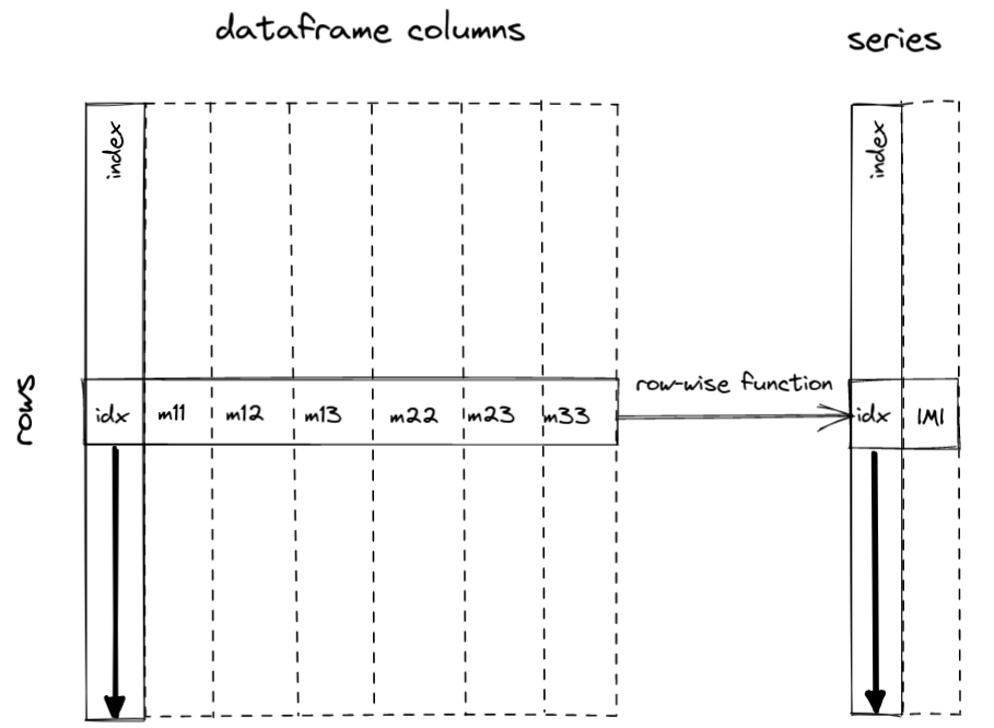
The focus is on looping over the rows of a Pandas dataframe holding some numerical data. All the elements of the dataframe are of np.float64 data type. A function is applied to each row, taking the row elements as input, either as distinct scalar arguments, as an array, or as a Pandas Series. The computation returns a scalar value per row, so that the process eventually returns a numeric Pandas series with same index as the original dataframe. For this post, a toy function computing the determinant of a 3-by-3 symmetric real matrix is used:
Here is a pure python implementation of the row-wise function:
def det_sym33(m11, m12, m13, m22, m23, m33):
    """Compute the determinant of a real symmetric 3x3 matrix
    given its 6 upper triangular coefficients.
    """
    return (
        m11 * (m22 * m33 - m23**2)
        + m12 * (2.0 * m23 * m13 - m12 * m33)
        - m22 * m13**2
    )
Imports
from itertools import cycle
from time import perf_counter

import cython
import dask.dataframe as dd
from numba import jit, float64, njit, prange
import numpy as np
import perfplot
import pandas as pd
import polars as pl
import swifter

%load_ext Cython
%load_ext line_profiler

SD = 124  # random seed
rng = np.random.default_rng(SD)  # random number generator
Python version       : 3.9.10
IPython version      : 8.0.1
polars    : 0.12.19
numpy     : 1.21.5
swifter   : 1.0.9
pandas    : 1.4.1
cython    : 0.29.28
numba     : 0.55.1
perfplot  : 0.10.1
dask      : 2022.2.1
Computations are performed on a laptop with an 8 cores Intel i7-7700HQ CPU @ 2.80GHz, running Linux.
Timing function
This function is returning the best elapsed time over r trials, and the result of the computation:
def timing(func, df, r=10):
    timings = []
    for i in range(r):
        start = perf_counter()
        s = func(df)
        end = perf_counter()
        elapsed_time = end - start
        timings.append(elapsed_time)
    return s, np.amin(timings)
Create a dataframe with random floats
We start by creating a medium-sized dataframe to perform a first comparison. We will later compare the most efficient methods with longer dataframes.
%%time
n = 100_000  # dataframe length
column_names = ['m11', 'm12', 'm13', 'm22', 'm23', 'm33']
df = pd.DataFrame(data=rng.random((n, 6)), columns=column_names)
CPU times: user 10.2 ms, sys: 143 µs, total: 10.4 ms
Wall time: 7.99 ms
df.head(3)
| m11 | m12 | m13 | m22 | m23 | m33 | |
|---|---|---|---|---|---|---|
| 0 | 0.785253 | 0.785859 | 0.969136 | 0.748060 | 0.655551 | 0.938885 |
| 1 | 0.178614 | 0.588647 | 0.442799 | 0.348847 | 0.330929 | 0.159369 |
| 2 | 0.989463 | 0.257111 | 0.715765 | 0.505885 | 0.664111 | 0.702342 |
Row-wise functions
We now create 3 different row-wise functions, with different argument types for the input row values:
- distinct scalar arguments
- an array
- a Pandas Series
def det_sym33_scalars(m11, m12, m13, m22, m23, m33):
    return (
        m11 * (m22 * m33 - m23**2)
        + m12 * (2.0 * m23 * m13 - m12 * m33)
        - m22 * m13**2
    )
def det_sym33_array(m):
    return (
        m[0] * (m[3] * m[5] - m[4] ** 2)
        + m[1] * (2.0 * m[4] * m[2] - m[1] * m[5])
        - m[3] * m[2] ** 2
    )
def det_sym33_series(s):
    return (
        s.m11 * (s.m22 * s.m33 - s.m23**2)
        + s.m12 * (2.0 * s.m23 * s.m13 - s.m12 * s.m33)
        - s.m22 * s.m13**2
    )
In the following, we may try several of these row-wise functions for a given dataframe looping method, depending on how the dataframe rows are returned by the method.
Pandas built-in vectorization
First we are going to use the built-in vectorization operations from Pandas. In the present case the row-wise computation is straightforward and can be performed with basic universal functions applied to the entire columns. This does not make use of any row-wise function, but allows us to have a reference timing.
def pandas_vectorize(df):
    return (
        df.m11 * (df.m22 * df.m33 - df.m23**2)
        + df.m12 * (2.0 * df.m23 * df.m13 - df.m12 * df.m33)
        - df.m22 * df.m13**2
    )
We store the resulting Pandas Series into the det_ref variable, in order to check that the later computations lead to the same result:
det_ref, t = timing(pandas_vectorize, df)
print(f"Elapsed time: {t:8.7f} s")
Elapsed time: 0.0044875 s
pandas.DataFrame.iterrows
We know that the iterrows method is kind of slow (see the previous post for example). It loops over dataframe rows as (index, Series) pairs. Here, we are going to compare the 3 different argument types of the row-wise function, given that the row returned by iterrows is a Pandas Series:
- scalar values
- a Numpy array
- a Pandas Series
| function name | method | returning rows as | row-wise function | argument type |
|---|---|---|---|---|
| iterrows_scalars | pd.DataFrame.iterrows | pd.Series | df_iterrows_scalars | float64 |
| iterrows_array | pd.DataFrame.iterrows | pd.Series | df_iterrows_array | array |
| iterrows_series | pd.DataFrame.iterrows | pd.Series | df_iterrows_series | pd.Series |
Scalar arguments
def iterrows_scalars(df):
    det = np.zeros(len(df), dtype=np.float64)
    i = 0
    for _, row in df.iterrows():
        det[i] = det_sym33_scalars(row.m11, row.m12, row.m13, row.m22, row.m23, row.m33)
        i += 1
    return pd.Series(det, index=df.index)
det, t_scalars = timing(iterrows_scalars, df, r=3)
print(f"Elapsed time: {t_scalars:8.7f} s")
Elapsed time: 5.6840575 s
pd.testing.assert_series_equal(det, det_ref)
numpy.ndarray argument
def iterrows_array(df):
    det = np.zeros(len(df), dtype=np.float64)
    i = 0
    for _, row in df.iterrows():
        det[i] = det_sym33_array(row.values)
        i += 1
    return pd.Series(det, index=df.index)
det, t_array = timing(iterrows_array, df, r=3)
print(f"Elapsed time: {t_array:8.7f} s")
Elapsed time: 2.4847183 s
pd.testing.assert_series_equal(det, det_ref)
pandas.Series argument
def iterrows_series(df):
    det = np.zeros(len(df), dtype=np.float64)
    i = 0
    for _, row in df.iterrows():
        det[i] = det_sym33_series(row)
        i += 1
    return pd.Series(det, index=df.index)
det, t_series = timing(iterrows_series, df, r=3)
print(f"Elapsed time: {t_series:8.7f} s")
Elapsed time: 7.8285359 s
pd.testing.assert_series_equal(det, det_ref)
Comparison
ax = (
    pd.DataFrame(
        data=[{"scalars": t_scalars, "array": t_array, "Series": t_series}],
        index=["elapsed_time"],
    )
    .T.sort_values(by="elapsed_time", ascending=False)
    .plot.bar(legend=False, alpha=0.75, rot=45)
)
_ = ax.set(
    title="iterrows() with 3 different argument types",
    xlabel="Argument type",
    ylabel="Elapsed time (s)",
)
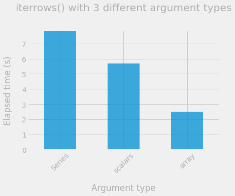
We observe that using the array of values from the pandas.Series as argument of the row-wise function, and accessing the data with indices is the fastest method when using .iterrows(). However, all three iterrows methods are very slow.
pandas.DataFrame.apply
The apply method also iterates over dataframe rows (with the axis=1 argument), returning either a Series (default) or an array (with raw=True). Here is what Pandas’ documentation says about it:
the passed function will receive ndarray objects instead. If you are just applying a NumPy reduction function this will achieve much better performance.
| function name | method | returning rows as | row-wise function | argument type |
|---|---|---|---|---|
| apply_series | pd.DataFrame.apply | pd.Series | det_sym33_series | pd.Series |
| apply_array | pd.DataFrame.apply | np.ndarray | det_sym33_array | array |
pandas.Series argument
def apply_series(df):
    return df.apply(det_sym33_series, raw=False, axis=1)
det, t_series = timing(apply_series, df, r=3)
print(f"Elapsed time: {t_series:8.7f} s")
Elapsed time: 5.1164269 s
pd.testing.assert_series_equal(det, det_ref)
numpy.ndarray argument
def apply_array(df):
    return df.apply(det_sym33_array, raw=True, axis=1)
det, t_array = timing(apply_array, df, r=3)
print(f"Elapsed time: {t_array:8.7f} s")
Elapsed time: 0.2638231 s
pd.testing.assert_series_equal(det, det_ref)
Comparison
ax = (
    pd.DataFrame(
        data=[{"array": t_array, "Series": t_series}],
        index=["elapsed_time"],
    )
    .T.sort_values(by="elapsed_time", ascending=False)
    .plot.bar(legend=False, alpha=0.75, rot=45)
)
_ = ax.set(
    title="apply() with 2 different argument types",
    xlabel="Argument type",
    ylabel="Elapsed time (s)",
)
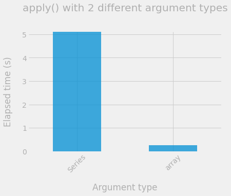
Indeed using arrays instead of Series is way faster! But still a lot slower than pandas built-in vectorization.
pandas.DataFrame.itertuples
The itertuples method allows the iteratation over dataframe rows, returning them as namedtuples. Thus, the row values can either be accessed by name or by index. The function det_sym33_scalars and det_sym33_series are used in the former case, and det_sym33_array in the latter.
| function name | method | returning rows as | row-wise function | argument type |
|---|---|---|---|---|
| itertuples_scalars | pd.DataFrame.itertuples | namedtuple | det_sym33_scalars | float64 |
| itertuples_array | pd.DataFrame.itertuples | namedtuple | det_sym33_array | array |
| itertuples_series | pd.DataFrame.itertuples | namedtuple | det_sym33_series | pd.Series |
Scalar arguments
def itertuples_scalars(df):
    det = np.zeros(len(df), dtype=np.float64)
    i = 0
    for row in df.itertuples():
        det[i] = det_sym33_scalars(row.m11, row.m12, row.m13, row.m22, row.m23, row.m33)
        i += 1
    return pd.Series(det, index=df.index)
det, t_scalars = timing(itertuples_scalars, df)
print(f"Elapsed time: {t_scalars:8.7f} s")
Elapsed time: 0.1051879 s
pd.testing.assert_series_equal(det, det_ref)
numpy.array argument
When row values are accessed by index, we need to account for the dataframe index, which is indexed by 0.
def itertuples_array(df):
    det = np.zeros(len(df), dtype=np.float64)
    i = 0
    for row in df.itertuples():
        det[i] = det_sym33_array(row[1:])
        i += 1
    return pd.Series(det, index=df.index)
det, t_array = timing(itertuples_array, df)
print(f"Elapsed time: {t_array:8.7f} s")
Elapsed time: 0.1136810 s
pd.testing.assert_series_equal(det, det_ref)
pandas.Series argument
def itertuples_series(df):
    det = np.zeros(len(df), dtype=np.float64)
    i = 0
    for row in df.itertuples():
        det[i] = det_sym33_series(row)
        i += 1
    return pd.Series(det, index=df.index)
det, t_series = timing(itertuples_series, df)
print(f"Elapsed time: {t_series:8.7f} s")
Elapsed time: 0.1084384 s
pd.testing.assert_series_equal(det, det_ref)
Comparison
ax = (
    pd.DataFrame(
        data=[{"scalars": t_scalars, "array": t_array, "Series": t_series}],
        index=["elapsed_time"],
    )
    .T.sort_values(by="elapsed_time", ascending=False)
    .plot.bar(legend=False, alpha=0.75, rot=45)
)
_ = ax.set(
    title="itertuples() with 3 different argument types",
    xlabel="Argument type",
    ylabel="Elapsed time (s)",
)
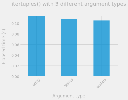
We get kind of similar results with the 3 different argument types. Once again, we can say than itertuples is to be prefered over iterrows and apply.
numpy.apply_along_axis
Let’s try out this method allowing to apply a function to a 1D slice along a given axis (rows of a 2D array in our case).
| function name | method | returning rows as | row-wise function | argument type |
|---|---|---|---|---|
| np_apply_along_axis | np.apply_along_axis | np.ndarray | det_sym33_array | array |
def np_apply_along_axis(df):

    return pd.Series(
        np.apply_along_axis(func1d=det_sym33_array, axis=1, arr=df.values),
        index=df.index,
    )
det, t = timing(np_apply_along_axis, df)
print(f"Elapsed time: {t:8.7f} s")
Elapsed time: 0.2435897 s
pd.testing.assert_series_equal(det, det_ref)
Well this is rather slow and disapointing…
numpy.vectorize
Numpy vectorize evaluates the row-wise function over each element of the input numpy array(s). However, note the warning on the NumPy documentation:
The vectorize function is provided primarily for convenience, not for performance. The implementation is essentially a for loop.
| function name | method | returning rows as | row-wise function | argument type |
|---|---|---|---|---|
| np_vectorize_scalars | np.vectorize | float64 | det_sym33_scalars | float64 |
| np_vectorize_array | np.vectorize | np.ndarray | det_sym33_array | array |
Scalar arguments
def np_vectorize_scalars(df):

    return pd.Series(
        np.vectorize(det_sym33_scalars)(df.m11, df.m12, df.m13, df.m22, df.m23, df.m33),
        index=df.index,
    )
det, t_scalars = timing(np_vectorize_scalars, df)
print(f"Elapsed time: {t_scalars:8.7f} s")
Elapsed time: 0.0498839 s
pd.testing.assert_series_equal(det, det_ref)
numpy.ndarray argument
In this case we need to add a signature argument in order to specify the input shape of the row-wise function.
def np_vectorize_array(df):

    return pd.Series(
        np.vectorize(det_sym33_array, signature="(n)->()")(
            df[["m11", "m12", "m13", "m22", "m23", "m33"]].values
        ),
        index=df.index,
    )
det, t_array = timing(np_vectorize_array, df)
print(f"Elapsed time: {t_array:8.7f} s")
Elapsed time: 0.2720111 s
pd.testing.assert_series_equal(det, det_ref)
Comparison
ax = (
    pd.DataFrame(
        data=[{"scalars": t_scalars, "array": t_array}],
        index=["elapsed_time"],
    )
    .T.sort_values(by="elapsed_time", ascending=False)
    .plot.bar(legend=False, alpha=0.75, rot=45)
)
_ = ax.set(
    title="numpy.vectorize() with 2 different argument types",
    xlabel="Argument type",
    ylabel="Elapsed time (s)",
)
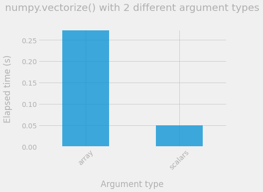
The version with scalar arguments is quite interesting, faster than itertuples.
map
Let’s use the standard map() Python method.
| function name | method | returning rows as | row-wise function | argument type |
|---|---|---|---|---|
| map_scalars | map | float64 | det_sym33_scalars | float64 |
def map_scalars(df):
    return pd.Series(
        map(det_sym33_scalars, df.m11, df.m12, df.m13, df.m22, df.m23, df.m33),
        index=df.index,
    )
det, t = timing(map_scalars, df)
print(f"Elapsed time: {t:8.7f} s")
Elapsed time: 0.0679905 s
pd.testing.assert_series_equal(det, det_ref)
Performance seems to be similar between map_scalars and np_vectorize_scalars.
Swifter
Swifter is a “package which efficiently applies any function to a pandas dataframe or series in the fastest available manner”. we use the raw=True argument. Here is a quote from the documentation :
raw : bool, default False
False : passes each row or column as a Series to the function.
True : the passed function will receive ndarray objects instead. If you are just applying a NumPy reduction function this will achieve much better performance.
| function name | method | returning rows as | row-wise function | argument type |
|---|---|---|---|---|
| swifter_apply | swifter.apply | np.ndarray | det_sym33_array | array |
def swifter_apply(df):
    return df.swifter.progress_bar(False).apply(det_sym33_array, raw=True, axis=1)
det, t = timing(swifter_apply, df)
print(f"Elapsed time: {t:8.7f} s")
Elapsed time: 0.2725223 s
pd.testing.assert_series_equal(det, det_ref)
The computation is rather slow, we are probably missing something here and did not use this package correctly?
dask.dataframe.map_partitions
We tried to use the great dask library with the map_partitions method. Unfortunately, we did not completely figure out how to handle the meta argument. Here is the description from the documentation:
meta : pd.DataFrame, pd.Series, dict, iterable, tuple, optional An empty pd.DataFrame or pd.Series that matches the dtypes and column names of the output. This metadata is necessary for many algorithms in dask dataframe to work. For ease of use, some alternative inputs are also available. Instead of a DataFrame, a dict of {name: dtype} or iterable of (name, dtype) can be provided (note that the order of the names should match the order of the columns). Instead of a series, a tuple of (name, dtype) can be used. If not provided, dask will try to infer the metadata. This may lead to unexpected results, so providing meta is recommended. For more information, see dask.dataframe.utils.make_meta.
The following implementation does work but there might be more efficient ways to do it…
| function name | method | returning rows as | row-wise function | argument type |
|---|---|---|---|---|
| dask_df_map_partitions | dd.map_partitions | pd.Series | det_sym33_series | pd.Series |
def dask_df_map_partitions(df, n_jobs=8):
    ddf = dd.from_pandas(df, npartitions=n_jobs)
    return pd.Series(
        ddf.map_partitions(
            det_sym33_series, meta=pd.Series(dtype=np.float64)
        ).compute(),
        index=df.index,
    )
det, t = timing(dask_df_map_partitions, df)
print(f"Elapsed time: {t:8.7f} s")
Elapsed time: 0.0254871 s
pd.testing.assert_series_equal(det, det_ref)
Not so bad but still slower than Pandas built_in vectorization. Here is what can be found on dask’s documentaion:
Note that, despite parallelism, Dask.dataframe may not always be faster than Pandas. We recommend that you stay with Pandas for as long as possible before switching to Dask.dataframe.
Also, we guess that there might be a dataframe copy from Pandas to Dask? This method is probably more recommended when dealing with very large dataframes distributed on clusters.
polars.DataFrame.apply
Polars is a fast multi-threaded DataFrame library written in Rust but also available in Python and Node.js. Here we are going to use DataFrame.apply() which allows to apply a custom function over the rows of a Polars dataFrame. The rows are passed as tuple. However, note this warning from Polars’ documentation:
Beware, this is slow.
| function name | method | returning rows as | row-wise function | argument type |
|---|---|---|---|---|
| polars_apply | polars.DataFrame.apply() | tuple | det_sym33_array | array |
def polars_apply(df):
    df_pl = pl.from_pandas(df)
    det_pl = df_pl.apply(det_sym33_array)
    det_pd = det_pl.to_pandas()["apply"]
    det_pd.index = df.index
    det_pd.name = None
    return det_pd
det, t = timing(polars_apply, df)
print(f"Elapsed time: {t:8.7f} s")
Elapsed time: 0.0902959 s
pd.testing.assert_series_equal(det, det_ref)
This is not so bad but one can wonder if a large part of the elapsed time is not spent converting the dataframe from Pandas to Polars and backward. Let’s measure the elepased time per line with a line profiler:
%lprun -f polars_apply polars_apply(df)
Timer unit: 1e-06 s

Total time: 0.229353 s
File: /tmp/ipykernel_16266/3940900507.py
Function: polars_apply at line 1

Line #      Hits         Time  Per Hit   % Time  Line Contents
==============================================================
     1                                           def polars_apply(df):
     2         1       6545.0   6545.0      2.9      df_pl = pl.from_pandas(df)
     3         1     221243.0 221243.0     96.5      det_pl = df_pl.apply(det_sym33_array)
     4         1       1542.0   1542.0      0.7      det_pd = det_pl.to_pandas()["apply"]
     5         1         14.0     14.0      0.0      det_pd.index = df.index
     6         1          9.0      9.0      0.0      det_pd.name = None
     7         1          0.0      0.0      0.0      return det_pd
Most of the time is actually spent within the apply method. However, we believe that there is a copy process in the from_pandas step, which would not be not optimal regarding memory usage?
Polars vectorize
We can also use Polars built-in vectorization the same way we did with Pandas. This does not make use of the previous row-wise functions.
def polars_vectorize(df):
    df_pl = pl.from_pandas(df)
    det_pl = (
        df_pl.m11 * (df_pl.m22 * df_pl.m33 - df_pl.m23**2)
        + df_pl.m12 * (2.0 * df_pl.m23 * df_pl.m13 - df_pl.m12 * df_pl.m33)
        - df_pl.m22 * df_pl.m13**2
    )
    det_pd = det_pl.to_frame().to_pandas()["m11"]
    det_pd.index = df.index
    det_pd.name = None
    return det_pd
det, t = timing(polars_vectorize, df)
print(f"Elapsed time: {t:8.7f} s")
Elapsed time: 0.0090223 s
pd.testing.assert_series_equal(det, det_ref)
If we run the line profiler, we can observe that most of the elapsed time is now spent converting the dataframe between Pandas and polars:
%lprun -f polars_vectorize polars_vectorize(df)
Timer unit: 1e-06 s

Total time: 0.014961 s
File: /tmp/ipykernel_16266/1430159236.py
Function: polars_vectorize at line 1

Line #      Hits         Time  Per Hit   % Time  Line Contents
==============================================================
     1                                           def polars_vectorize(df):
     2         1       7295.0   7295.0     48.8      df_pl = pl.from_pandas(df)
     3         1          1.0      1.0      0.0      det_pl = (
     4         3       2915.0    971.7     19.5          df_pl.m11 * (df_pl.m22 * df_pl.m33 - df_pl.m23**2)
     5         1        551.0    551.0      3.7          + df_pl.m12 * (2.0 * df_pl.m23 * df_pl.m13 - df_pl.m12 * df_pl.m33)
     6         1       2363.0   2363.0     15.8          - df_pl.m22 * df_pl.m13**2
     7                                               )
     8         1       1807.0   1807.0     12.1      det_pd = det_pl.to_frame().to_pandas()["m11"]
     9         1         17.0     17.0      0.1      det_pd.index = df.index
    10         1         11.0     11.0      0.1      det_pd.name = None
    11         1          1.0      1.0      0.0      return det_pd
Numba
Numba makes Python code fast! Here we use the Numba @jit decorator with nogil=True for the Numba dedicated row-wise function. In the apply_func_numba function, we basically implement the loop over the dataframe rows.
@jit(
    float64(float64, float64, float64, float64, float64, float64),
    nogil=True,
)
def det_sym33_numba(m11, m12, m13, m22, m23, m33):
    return (
        m11 * (m22 * m33 - m23**2)
        + m12 * (2.0 * m23 * m13 - m12 * m33)
        - m22 * m13**2
    )


@jit
def apply_func_numba(col_m11, col_m12, col_m13, col_m22, col_m23, col_m33):
    n = len(col_m11)
    det = np.empty(n, dtype="float64")
    for i in range(n):
        det[i] = det_sym33_numba(
            col_m11[i], col_m12[i], col_m13[i], col_m22[i], col_m23[i], col_m33[i]
        )
    return det


def numba_loop(df):
    det = apply_func_numba(
        df["m11"].to_numpy(),
        df["m12"].to_numpy(),
        df["m13"].to_numpy(),
        df["m22"].to_numpy(),
        df["m23"].to_numpy(),
        df["m33"].to_numpy(),
    )
    return pd.Series(det, index=df.index)
det, t = timing(numba_loop, df, r=100)
print(f"Elapsed time: {t:8.7f} s")
Elapsed time: 0.0002950 s
pd.testing.assert_series_equal(det, det_ref)
Well this is the fastest implementation so far.
Numba parallel
Now we use the Numba @njit decorator along with prange looping. By default, all available cores are used. The previous row-wise function apply_func_numba is used here.
@njit(parallel=True)
def apply_func_numba_para(col_m11, col_m12, col_m13, col_m22, col_m23, col_m33):
    n = len(col_m11)
    det = np.empty(n, dtype="float64")
    for i in prange(n):
        det[i] = det_sym33_numba(
            col_m11[i], col_m12[i], col_m13[i], col_m22[i], col_m23[i], col_m33[i]
        )
    return det


def numba_loop_para(df):
    det = apply_func_numba_para(
        df["m11"].to_numpy(),
        df["m12"].to_numpy(),
        df["m13"].to_numpy(),
        df["m22"].to_numpy(),
        df["m23"].to_numpy(),
        df["m33"].to_numpy(),
    )
    return pd.Series(det, index=df.index)
det, t = timing(numba_loop_para, df, r=100)
print(f"Elapsed time: {t:8.7f} s")
Elapsed time: 0.0002439 s
pd.testing.assert_series_equal(det, det_ref)
The parallel version is not a large improvement over the sequantial Numba version. This might be because of the relatively small size of the dataframe.
Cython
Cython is a mix between C and Python. Writing Cython code is a little more involving than writing pure Python. Note that in the following we used %%cython magic command at the begining of the notebook cell to compile the Cython code (also we loaded the Cython extension at the begining of the notebook).
%%cython

cimport cython
import numpy as np
import pandas as pd

@cython.binding(False)
@cython.boundscheck(False)
@cython.wraparound(False)
@cython.initializedcheck(False)
cdef void loop_cython(double[:] det, double[:] m11, double[:] m12, double[:] m13, double[:] m22, double[:] m23, double[:] m33) nogil:

    cdef Py_ssize_t i

    for i in range(m11.shape[0]):
        det[i] = m11[i] * (m22[i] * m33[i] - m23[i] ** 2) + m12[i] * (2.0 * m23[i] * m13[i] - m12[i] * m33[i]) - m22[i] * m13[i] ** 2


cpdef cython_loop(df):

    det = np.zeros_like(df.m11.values)
    loop_cython(det, df.m11.values, df.m12.values, df.m13.values, df.m22.values, df.m23.values, df.m33.values)

    return pd.Series(det, index=df.index)
det, t = timing(cython_loop, df, r=100)
print(f"Elapsed time: {t:8.7f} s")
Elapsed time: 0.0004649 s
pd.testing.assert_series_equal(det, det_ref)
This is not as fast as Numba but close.
Cython parallel
Similarly to what we did with Numba, we use here the prange looping function. Here is a quote from the documentation:
cython.parallel.prange([start,] stop[, step][, nogil=False][, schedule=None[, chunksize=None]][, num_threads=None])
This function can be used for parallel loops. OpenMP automatically starts a thread pool and distributes the work according to the schedule used. Thread-locality and reductions are automatically inferred for variables.
%%cython --compile-args=-fopenmp --link-args=-fopenmp

cimport cython
from cython.parallel import prange

import numpy as np
import pandas as pd

@cython.binding(False)
@cython.boundscheck(False)
@cython.wraparound(False)
@cython.initializedcheck(False)
cdef void loop_cython_para(double[:] det, double[:] m11, double[:] m12, double[:] m13, double[:] m22, double[:] m23, double[:] m33) nogil:

    cdef Py_ssize_t i

    for i in prange(m11.shape[0], nogil=True):
        det[i] = m11[i] * (m22[i] * m33[i] - m23[i] ** 2) + m12[i] * (2.0 * m23[i] * m13[i] - m12[i] * m33[i]) - m22[i] * m13[i] ** 2


cpdef cython_loop_para(df):

    det = np.zeros_like(df.m11.values)
    loop_cython_para(det, df.m11.values, df.m12.values, df.m13.values, df.m22.values, df.m23.values, df.m33.values)

    return pd.Series(det, index=df.index)
det, t = timing(cython_loop_para, df, r=100)
print(f"Elapsed time: {t:8.7f} s")
Elapsed time: 0.0003041 s
The parallel version is a little faster that the sequential one but we should test it on larger dataframes.
Global comparison
We start by comparing all methods over small size dataframes.
Small size dataframes
def compare_all_methods(rng, funcs, df_sizes):

    column_names = ["m11", "m12", "m13", "m22", "m23", "m33"]
    time_df = pd.DataFrame()
    for n in df_sizes:

        df = pd.DataFrame(data=rng.random((n, 6)), columns=column_names)

        d = {}
        for func in funcs:
            _, t = timing(func, df)
            d[func.__name__] = t
        df_tmp = pd.DataFrame(d, index=[n])
        time_df = pd.concat((time_df, df_tmp), axis=0)

    return time_df
funcs = [
    pandas_vectorize,
    iterrows_array,
    apply_array,
    itertuples_scalars,
    np_apply_along_axis,
    np_vectorize_scalars,
    map_scalars,
    swifter_apply,
    dask_df_map_partitions,
    polars_apply,
    polars_vectorize,
    numba_loop,
    numba_loop_para,
    cython_loop,
    cython_loop_para,
]


time_df = compare_all_methods(rng, funcs, df_sizes=[1_000, 10_000])
c_max = time_df.iloc[-1]
c_max = c_max.sort_values(ascending=False)
columns = c_max.index.values.tolist()
time_df = time_df[columns]
ax = time_df.plot.bar(stacked=False, figsize=(16, 8), logy=True, rot=0)
_ = ax.set_ylim(1.0e-5)
_ = ax.set(
    title="Timing comparison of various dataframe looping methods",
    xlabel="Dataframe length",
    ylabel="Elapsed_time [s] (log scale)",
)
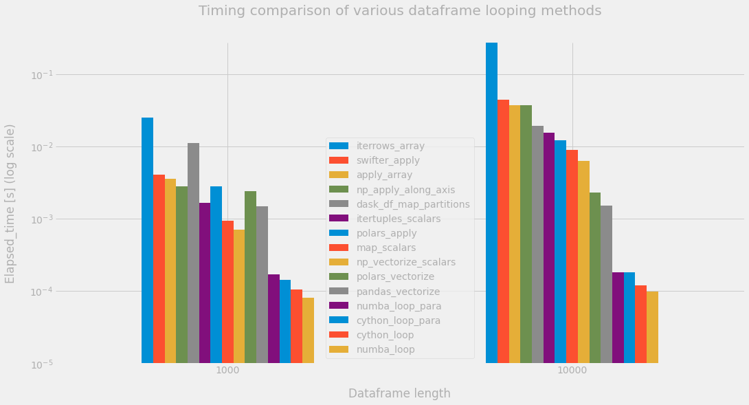
Only the Numba and Cython methods are significantly faster than Pandas’ built_in vectorization (pandas_vectorize)!
pd.options.display.float_format = "{:,.2e}".format
time_df.T
| 1000 | 10000 | |
|---|---|---|
| iterrows_array | 2.50e-02 | 2.76e-01 |
| swifter_apply | 4.08e-03 | 4.41e-02 |
| apply_array | 3.56e-03 | 3.75e-02 |
| np_apply_along_axis | 2.79e-03 | 3.71e-02 |
| dask_df_map_partitions | 1.11e-02 | 1.92e-02 |
| itertuples_scalars | 1.66e-03 | 1.56e-02 |
| polars_apply | 2.82e-03 | 1.21e-02 |
| map_scalars | 9.42e-04 | 9.08e-03 |
| np_vectorize_scalars | 7.03e-04 | 6.39e-03 |
| polars_vectorize | 2.39e-03 | 2.30e-03 |
| pandas_vectorize | 1.50e-03 | 1.52e-03 |
| numba_loop_para | 1.68e-04 | 1.84e-04 |
| cython_loop_para | 1.43e-04 | 1.81e-04 |
| cython_loop | 1.06e-04 | 1.20e-04 |
| numba_loop | 8.01e-05 | 9.84e-05 |
Medium to large size dataframes
funcs = [
    pandas_vectorize,
    numba_loop,
    numba_loop_para,
    cython_loop,
    cython_loop_para,
]


time_df = compare_all_methods(rng, funcs, df_sizes=[1_000_000, 10_000_000])
c_max = time_df.iloc[-1]
c_max = c_max.sort_values(ascending=False)
columns = c_max.index.values.tolist()
time_df = time_df[columns]
ax = time_df.plot.bar(stacked=False, figsize=(16, 8), logy=True, rot=0)
_ = ax.set_ylim(1.0e-5)
_ = ax.set(
    title="Timing comparison of various dataframe looping methods",
    xlabel="Dataframe length",
    ylabel="Elapsed_time [s] (log scale)",
)
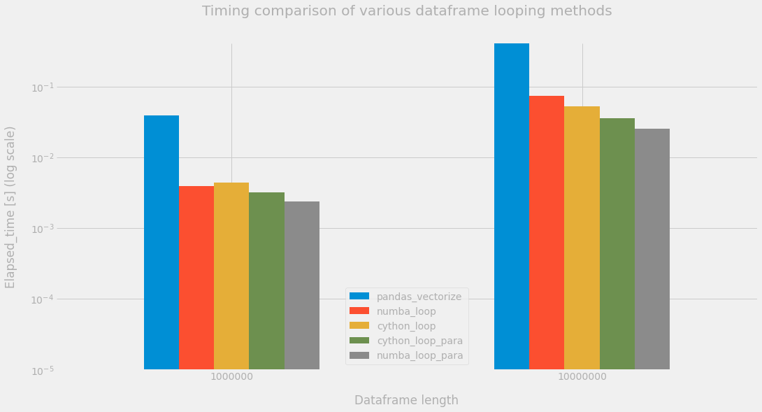
time_df.T
| 1000000 | 10000000 | |
|---|---|---|
| pandas_vectorize | 3.95e-02 | 4.10e-01 |
| numba_loop | 3.92e-03 | 7.33e-02 |
| cython_loop | 4.40e-03 | 5.29e-02 |
| cython_loop_para | 3.21e-03 | 3.55e-02 |
| numba_loop_para | 2.35e-03 | 2.53e-02 |
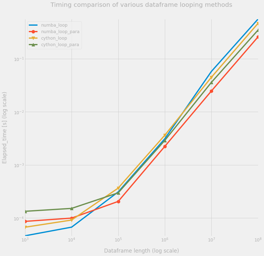
Let’s focus on the Numba and Cython methods.
funcs = [
    numba_loop,
    numba_loop_para,
    cython_loop,
    cython_loop_para,
]

out = perfplot.bench(
    setup=lambda n: pd.DataFrame(data=rng.random((n, 6)), columns=column_names),
    kernels=[(lambda df: func)(df) for func in funcs],
    labels=[func.__name__ for func in funcs],
    n_range=[10**k for k in range(3, 9)],
)
def plot_timings(out, figsize=(12,12)):
    labels = out.labels
    ms = 10
    fig = plt.figure(figsize=figsize)
    ax = fig.add_subplot(1, 1, 1)

    for i, label in enumerate(labels):
        plt.loglog(out.n_range, out.timings_s[i], "o-", ms=ms, label=label)
    markers = cycle(
        ("", "o", "v", "^", "<", ">", "s", "p", "P", "*", "h", "X", "D", ".")
    )
    for i, line in enumerate(ax.get_lines()):
        marker = next(markers)
        line.set_marker(marker)
    plt.legend()
    plt.grid("on")
    _ = ax.set(
        title="Timing comparison of various dataframe looping methods",
        xlabel="Dataframe length (log scale)",
        ylabel="Elapsed_time [s] (log scale)",
    )

    return ax
ax = plot_timings(out)
Conclusion
Pandas built-in vectorization is a very good solution when possible. If we want to be faster with no extra pain, Numba is the best solution. Cython is about as fast as Numba, flexible, but more involving.