Heapsort with Numba and Cython
Updated April 20, 2022 following usefull comments by @scoder. Thank you very much for your pull requests!
Heapsort is a classical sorting algorithm. We are going into a little bit of theory about the algorithm, but refer to Corman et al. [1] for more details, or the heapsort wikipedia page.
In this post, we are going to implement the classical heapsort in Python, Python/Numba and Cython. The regular implementation is array-based and performed in-place. We use 0-based indices. Note that this is not a stable sorting method (keeping items with the same key in the original order).
Imports
from itertools import cycle

from binarytree import build
import cython
from numba import njit
import numpy as np
import perfplot
%load_ext cython

SD = 124  # random seed
rng = np.random.default_rng(SD)  # random number generator
Language/package versions:
Python implementation: CPython
Python version       : 3.9.12
IPython version      : 8.2.0
binarytree           : 6.5.1
matplotlib           : 3.5.1
perfplot             : 0.10.2
numpy                : 1.21.5
cython               : 0.29.28
numba                : 0.55.1
Float array creation
We assume that we want to sort an NumPy array of 64-bit floating-point numbers :
n = 10
A = rng.random(n, dtype=np.float64)
A
array([0.78525311, 0.78585936, 0.96913602, 0.74805977, 0.65555081,
       0.93888454, 0.17861445, 0.58864721, 0.44279917, 0.34884712])
Binary trees
Heapsort is based on binary heap data structure, which relies on a nearly complete binary tree:
a [nearly] complete binary tree is a binary tree in which every level, except possibly the last, is completely filled, and all nodes in the last level are as far left as possible.
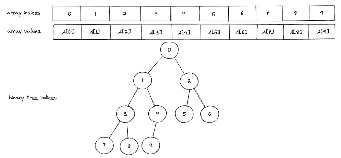
In a binary heap, the elements in an array are mapped to the tree nodes of a virtual binary tree. Assuming that we know the maximum number of elements in the heap, the array representation of the tree is more convenient than a linked structure. Note that it is also possible to use and array that can grow or shrink dynamically when threshold sizes are reached. Here is a figure showing the array elements and the corresponding tree nodes:

So we can see the array as a representation of the tree (implicit data structure): the node at the top (A[0]) of the tree is called the root, and the ones at the bottom, without children, are called the leaves (A[5], A[6], A[7], A[8], A[9]). An advantage of binary trees is that it is easy to navigate among the nodes. Tree node indexing goes from the root to the leaves and from left to right. Level $k\geq 0$ goes from node $2^k -1$ to node $2 (2^k -1)$. Within a level, you can go left by decrementing, and right by incrementing the node index by one. A node may have two children : the left and right ones. Given a node index i, the parent node index can be easily found as (i - 1) // 2:
def parent(i):
    assert i > 0
    return (i - 1) // 2
parent(1)
0
parent(8)
3
The left child has index 2 * i + 1 and the right child 2 * (i + 1):
def left_child(i):
    return 2 * i + 1


def right_child(i):
    return 2 * (i + 1)
left_child(0)
1
right_child(0)
2
The depth of a node is the number of edges from the root node to the target node. The height $h$ of a binary tree is the number of edges from the root to the most distant leaf node (in the above example, the height is equal to 3). We can bound the number of elements $n$ of the nearly complete tree using its height:
\[2^h = \sum_{k=0}^{h-1} 2^k +1 \leq n \leq \sum_{k=0}^h 2^k = 2^{h+1}-1\]So that we have $h = \lfloor \log_2 n \rfloor $
Binary heap
Here is the definition of a heap [2]:
A heap is a set of nodes with keys arranged in a complete heap-ordered binary tree, represented as an array.
A binary heap is binary tree data structure that satisfies a heap property. There are two kinds of heaps : min- and max-heaps satisfying respectively a min-heap or a max-heap property. In our case, we are going to use a max-heap to easily implement the heapsort algorithm. A min-heap would be used if sorting the array in a descending order, or would imply extra space/work to sort in ascending order.
max-heap property : A value of a given node i is not larger than the value of its parent node parent(i)
Thus value of the root node A[0] of a max-heap is greater than or equal to all the tree values. This is also true for any sub-tree of the binary heap: the root node of any sub-tree A[i] is greater than or equal to all the values in this sub-tree.
An important point is that not all the array elements might be in the heap. We differentiate the heap size from the array length $n$. We have $0 \leq size \leq n$. The element in heap are the size elements in the left part of the array: A[0:size] (with a Python slicing indexing). All remaining elements A[size:n] are not in the heap, implicitely.
Initially, given the above array A, it mostly likely does not satisfy the max-heap property, which would imply in our case:
A[0] >= A[1], A[0] >= A[2], A[1] >= A[3], A[1] >= A[4], A[3] >= A[7], A[3] >= A[8 ], A[2] >= A[5], A[2] >= A[6]. Indeed we have:
A[0] >= A[1]
False
A[0] >= A[2]
False
We need to build the max-heap from an array by moving around the elements. In order to do that, we use a function called max_heapify from the leaves to the root of the tree, in a bottom-up manner. So let’s implement this function.
Max_heapify
The max_heapify(A, size, i) function presupposes that sub-trees rooted at the children nodes of i do satisfy the max-heap property. But the i-th node may violate it, i.e. A[i] < A[left_child(i)] or A[i] < A[right_child(i)], assuming that the children are in the heap. If this is the case, the i-th node is swapped with its child with largest value:
A[i], A[largest] = A[largest], A[i]
This process is then repeated from the largest children node. Eventually, the sub-tree rooted at i satisfies the max-heap property after a call to max_heapify(A, size, i).
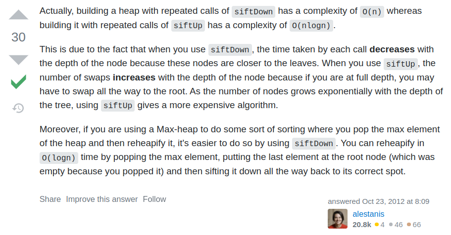
This process is also refered to as sift down: move a value violating the max-heap property down the tree by exchanging it with the largest of its 2 children values. Now it would also be possible to use the exact opposite process: sift up, which would start from a leaf node, and move its value up the tree by exchanging it with the parent node value, if violating the max-heap property. However, building a max-heap with the sift up process has a larger complexity than with sift down. I found this explanation by @alestanis on Stack Overflow really clear (The question was Why siftDown is better than siftUp in heapify?):

So here is a Python implementation:
def max_heapify(A, size, node_idx=0):

    largest = node_idx
    l = left_child(largest)
    r = right_child(largest)

    if (l < size) and (A[l] > A[largest]):
        largest = l

    if (r < size) and (A[r] > A[largest]):
        largest = r

    if largest != node_idx:
        A[node_idx], A[largest] = A[largest], A[node_idx]  # exchange 2 nodes
        max_heapify(A, size, largest)
Note that this function is recursive. Let’s have a look at the tree values of our example:
tree_values = build(list(A.round(5)))
print(tree_values)
                            ___________________0.78525___________
                           /                                     \
             __________0.78586___________                   ___0.96914___
            /                            \                 /             \
     ___0.74806__                   ___0.65555         0.93888         0.17861
    /            \                 /
0.58865         0.4428         0.34885
This array is random, but we can observe that the max-heap property is satisfied everywhere except at the root! The sub-trees rooted at nodes 1 and 2 do happen to satisfy the max-heap property already. So let’s call the max_heapify function on the root node.
max_heapify(A, len(A), node_idx=0)
tree_values = build(list(A.round(5)))
print(tree_values)
                            ___________________0.96914___________
                           /                                     \
             __________0.78586___________                   ___0.93888___
            /                            \                 /             \
     ___0.74806__                   ___0.65555         0.78525         0.17861
    /            \                 /
0.58865         0.4428         0.34885
The root node A[0] = 0.78525 moved from node index 0 to 2, and then from 2 to 5. Nodes 2 and 5 moved one step up in the process.
Steps:
- node 0 is compared with nodes 1 and 2. Node 0 is smaller than one of its children (0.78525 < 0.96914). Node 2 is the child with largest value : exchange node 0 and 2.
- node 2 is compared with nodes 5 and 6. Node 0 is smaller than one of its children (0.78525 < 0.93888). Node 5 is the child with largest value : exchange node 2 and 5.
- Node 5 is a leaf, so stop.
Let’s generate a new random array to see another example:
A = rng.random(n, dtype=np.float64)
A
array([0.3309295 , 0.15936868, 0.98946349, 0.25711078, 0.71576487,
       0.50588512, 0.66411132, 0.70234247, 0.05208023, 0.06009649])
tree_values = build(list(A.round(5)))
print(tree_values)
                             __________________0.33093___________
                            /                                    \
             ___________0.15937__________                   ___0.98946___
            /                            \                 /             \
     ___0.25711___                  ___0.71576         0.50589         0.66411
    /             \                /
0.70234         0.05208         0.0601
If we start from the leaves toward the root, we can notice a max-heap violation at node 3. So we call max_heapify on that node:
max_heapify(A, len(A), node_idx=3)
tree_values = build(list(A.round(5)))
print(tree_values)
                             __________________0.33093___________
                            /                                    \
             ___________0.15937__________                   ___0.98946___
            /                            \                 /             \
     ___0.70234___                  ___0.71576         0.50589         0.66411
    /             \                /
0.25711         0.05208         0.0601
Now let’s take care of node 1:
max_heapify(A, len(A), node_idx=1)
tree_values = build(list(A.round(5)))
print(tree_values)
                             __________________0.33093___________
                            /                                    \
             ___________0.71576__________                   ___0.98946___
            /                            \                 /             \
     ___0.70234___                  ___0.15937         0.50589         0.66411
    /             \                /
0.25711         0.05208         0.0601
And finally we need to fix the root value:
max_heapify(A, len(A), node_idx=0)
tree_values = build(list(A.round(5)))
print(tree_values)
                             __________________0.98946___________
                            /                                    \
             ___________0.71576__________                   ___0.66411___
            /                            \                 /             \
     ___0.70234___                  ___0.15937         0.50589         0.33093
    /             \                /
0.25711         0.05208         0.0601
We actually built a max-heap manually. In the following let’s see the general method to build it.
Build_max_heap
The method used to build the max-heap with a sift-down-based heapify is called Floyd’s heap construction:
Floyd’s algorithm starts with the leaves, observing that they are trivial but valid heaps by themselves, and then adds parents. Starting with element n/2 and working backwards, each internal node is made the root of a valid heap by sifting down. The last step is sifting down the first element, after which the entire array obeys the heap property.
This bottom-up heap construction technique runs in $O(n)$ time. Here is a Python implementation:
def build_max_heap(A):
    size = len(A)
    node_idx = size // 2 - 1  # last non-leaf node index
    for i in range(node_idx, -1, -1):
        max_heapify(A, size, node_idx=i)
    return size
A = rng.random(n, dtype=np.float64)
A
array([0.94535273, 0.25035043, 0.40579395, 0.27596342, 0.30065296,
       0.36667218, 0.14878984, 0.34834079, 0.59713033, 0.99416357])
tree_values = build(list(A.round(5)))
print(tree_values)
                             ___________________0.94535___________
                            /                                     \
             ___________0.25035___________                   ___0.40579___
            /                             \                 /             \
     ___0.27596___                   ___0.30065         0.36667         0.14879
    /             \                 /
0.34834         0.59713         0.99416
_ = build_max_heap(A)
tree_values = build(list(A.round(5)))
print(tree_values)
                             ___________________0.99416___________
                            /                                     \
             ___________0.94535___________                   ___0.40579___
            /                             \                 /             \
     ___0.59713___                   ___0.30065         0.36667         0.14879
    /             \                 /
0.34834         0.27596         0.25035
Heapsort
The classical heapsort has two steps:
1 - build the heap
2 - destroy the heap by removing the root from the heap and moving it to the end of the heap $n$ times.
Step 2 corresponds to the following iterations:
- swap the root (largest element) with the last leaf
- remove the last leaf from the heap.
- heapify the root on the reduced heap.
The average and worst-case performance are $O(n\log n)$. Here is a Python implementation:
def heapsort(A_in):

    A = np.copy(A_in)

    # build a max heap
    size = build_max_heap(A)

    for i in range(size - 1, 0, -1):

        # swap the root (largest element) with the last leaf
        A[i], A[0] = A[0], A[i]

        # removing largest element from the heap
        size -= 1

        # call _max_heapify from the root on the heap with remaining elements
        max_heapify(A, size, node_idx=0)

    return A
n = 10
A = rng.random(n, dtype=np.float64)
A
array([0.18525118, 0.99313433, 0.78561885, 0.44814329, 0.85044505,
       0.86088208, 0.96716993, 0.17096352, 0.69956773, 0.8288503 ])
A_sorted_python = heapsort(A)
A_sorted_python
array([0.17096352, 0.18525118, 0.44814329, 0.69956773, 0.78561885,
       0.8288503 , 0.85044505, 0.86088208, 0.96716993, 0.99313433])
A_ref = np.sort(A)
np.testing.assert_array_equal(A_sorted_python, A_ref)
Let’s use Numba to make this Python code running fast.
Numba
@njit
def max_heapify_numba(A, size, node_idx=0):

    largest = node_idx
    left_child = 2 * node_idx + 1
    right_child = 2 * (node_idx + 1)

    if (left_child < size) and (A[left_child] > A[largest]):
        largest = left_child

    if (right_child < size) and (A[right_child] > A[largest]):
        largest = right_child

    if largest != node_idx:
        A[node_idx], A[largest] = A[largest], A[node_idx]  # exchange 2 nodes
        max_heapify_numba(A, size, largest)

@njit
def heapsort_numba(A_in):

    A = np.copy(A_in)

    # build a max heap
    size = len(A)
    node_idx = size // 2 - 1  # last non-leaf node index
    for i in range(node_idx, -1, -1):
        max_heapify_numba(A, size, node_idx=i)

    for i in range(size - 1, 0, -1):
        # swap the root (largest element) with the last leaf
        A[i], A[0] = A[0], A[i]

        # removing largest element from the heap
        size -= 1

        # call _max_heapify from the root on the heap with remaining elements
        max_heapify_numba(A, size)
    return A
A_sorted_numba = heapsort_numba(A)
A_sorted_numba
array([0.17096352, 0.18525118, 0.44814329, 0.69956773, 0.78561885,
       0.8288503 , 0.85044505, 0.86088208, 0.96716993, 0.99313433])
np.testing.assert_array_equal(A_sorted_numba, A_ref)
Cython
%%cython --compile-args=-Ofast

# cython: boundscheck=False, initializedcheck=False, wraparound=False

import cython
import numpy as np

from cython import ssize_t, double


@cython.exceptval(check=False)
@cython.nogil
@cython.cfunc
def _max_heapify(A: double[::1], size: ssize_t, node_idx: ssize_t) -> cython.void:
    largest: ssize_t = node_idx

    left_child = 2 * node_idx + 1
    right_child = 2 * (node_idx + 1)

    if left_child < size and A[left_child] > A[largest]:
        largest = left_child

    if right_child < size and A[right_child] > A[largest]:
        largest = right_child

    if largest != node_idx:
        A[node_idx], A[largest] = A[largest], A[node_idx]
        _max_heapify(A, size, largest)


@cython.exceptval(check=False)
@cython.nogil
@cython.cfunc
def _heapsort(A: double[::1]) -> cython.void:
    i: cython.int
    size: ssize_t = len(A)
    node_idx: ssize_t = size // 2 - 1

    for i in range(node_idx, -1, -1):
        _max_heapify(A, size, i)

    for i in range(size - 1, 0, -1):
        A[i], A[0] = A[0], A[i]
        size -= 1
        _max_heapify(A, size, 0)


@cython.ccall
def heapsort_cython(A_in):
    A = np.copy(A_in)
    _heapsort(A)
    return A
A_sorted_cython = heapsort_cython(A)
A_sorted_cython
array([0.17096352, 0.18525118, 0.44814329, 0.69956773, 0.78561885,
       0.8288503 , 0.85044505, 0.86088208, 0.96716993, 0.99313433])
np.testing.assert_array_equal(A_sorted_cython, A_ref)
Performance comparison
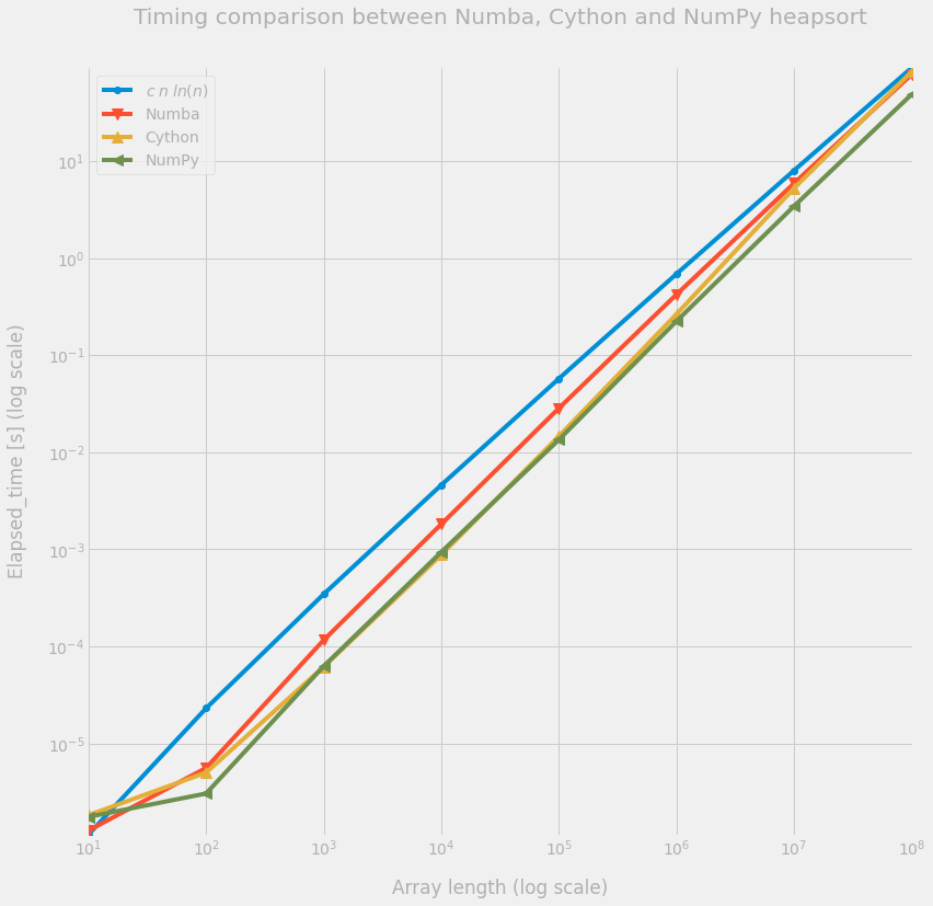
We do not include the Python version and compare the Numba and Cython versions with the NumPy heapsort implementation. It seems that this NumPy heapsort is written in C++ and is fairly well optimized.
out = perfplot.bench(
    setup=lambda n: rng.random(n, dtype=np.float64),
    kernels=[
        lambda A: heapsort_numba(A),
        lambda A: heapsort_cython(A),
        lambda A: np.sort(A, kind="heapsort"),
    ],
    labels=["Numba", "Cython", "NumPy"],
    n_range=[10**k for k in range(1, 9)],
)
out
┏━━━━━━━━━━━┳━━━━━━━━━━━━━━━━━━━━━┳━━━━━━━━━━━━━━━━━━━━━━━┳━━━━━━━━━━━━━━━━━━━━━━━━┓
┃ n         ┃ Numba               ┃ Cython                ┃ NumPy                  ┃
┡━━━━━━━━━━━╇━━━━━━━━━━━━━━━━━━━━━╇━━━━━━━━━━━━━━━━━━━━━━━╇━━━━━━━━━━━━━━━━━━━━━━━━┩
│ 10        │ 1.266e-06           │ 1.819e-06             │ 1.7500000000000002e-06 │
│ 100       │ 5.587e-06           │ 5.004000000000001e-06 │ 3.0430000000000003e-06 │
│ 1000      │ 0.000116266         │ 6.1561e-05            │ 6.2518e-05             │
│ 10000     │ 0.001819482         │ 0.0008792880000000001 │ 0.000939073            │
│ 100000    │ 0.028507956         │ 0.014659915           │ 0.013501216000000002   │
│ 1000000   │ 0.42401333100000005 │ 0.26564063200000004   │ 0.224838018            │
│ 10000000  │ 5.938197069         │ 5.285706523           │ 3.4547337810000003     │
│ 100000000 │ 78.544810064        │ 84.04674386900001     │ 49.002946636000004     │
└───────────┴─────────────────────┴───────────────────────┴────────────────────────┘
figsize = (14, 14)

labels = out.labels
ms = 10
fig = plt.figure(figsize=figsize)
ax = fig.add_subplot(1, 1, 1)
plt.loglog(
    out.n_range,
    out.n_range * np.log(out.n_range) * 5.0e-8,
    "o-",
    label="$c \; n \; ln(n)$",
)
for i, label in enumerate(labels):
    plt.loglog(out.n_range, out.timings_s[i], "o-", ms=ms, label=label)
markers = cycle(("o", "v", "^", "<", ">", "s", "p", "P", "*", "h", "X", "D", "."))
for i, line in enumerate(ax.get_lines()):
    marker = next(markers)
    line.set_marker(marker)
plt.legend()
plt.grid("on")
_ = ax.set(
    title="Timing comparison between Numba, Cython and NumPy heapsort",
    xlabel="Array length (log scale)",
    ylabel="Elapsed_time [s] (log scale)",
)

Conclusion
Going from Python to Numba is seamless and is allowing us to reach a similar level of efficiency as with Cython (that turned 20 years old last week, happy birthday!!). We can observe that the NumPy heapsort implementation is faster on larger arrays, but we do not know which optimizations did they implement.
References
[1] Thomas H. Cormen, Charles E. Leiserson, Ronald L. Rivest, and Clifford Stein. 2009. Introduction to Algorithms, Third Edition (3rd. ed.). The MIT Press.
[2] Robert Sedgewick. 2002. Algorithms in C (3rd. ed.). Addison-Wesley Longman Publishing Co., Inc., USA.