Reading a SQL table by chunks with Pandas
In this short Python notebook, we want to load a table from a relational database and write it into a CSV file. In order to that, we temporarily store the data into a Pandas dataframe. Pandas is used to load the data with read_sql() and later to write the CSV file with to_csv(). However, we have two constraints here:
-
we do not want to load the full table in memory. Indeed, Pandas is usually allocating a lot more memory than the table data size. That may be a problem if the table is rather large.
-
we want the process to be efficient, that is, not dramatically increase the running time when iterating over chunks as compared to loading the full table in memory.
In order to do that we are going to make use of two different things:
- An iterated loading process in Pandas, with a defined
chunksize.chunksizeis the number of rows to include in each chunk:
for df in pd.read_sql(sql_query, connection, chunksize=chunksize):
    do something
connection = engine.connect().execution_options(
    stream_results=True,
    max_row_buffer=chunksize)
Note that the result of the stream_results and max_row_buffer arguments might differ a lot depending on the database, DBAPI/database adapter. Here we load a table from PostgreSQL with the psycopg2 adapter. It seems that the server side cursor is the default with psycopg2 when using chunksize in pd.read_sql().
In the following, we are going to study how the elapsed time and max memory usage vary with respect to chunksize.
Imports
import urllib
from time import perf_counter

import matplotlib.pyplot as plt
import pandas as pd
from memory_profiler import memory_usage
from sqlalchemy import create_engine


PG_USERNAME = "***************"
PG_PASSWORD = "***************"
PG_SERVER = "localhost"
PG_PORT = 5432
PG_DATABASE = "test"
CONNECT_STRING = (
    f"postgresql+psycopg2://{PG_USERNAME}:"
    + f"{urllib.parse.quote_plus(PG_PASSWORD)}@{PG_SERVER}:{PG_PORT}/{PG_DATABASE}"
)

CSV_FP = "./test_01.csv"  # CSV file path
SQL_QUERY = """SELECT * FROM "faker_s1000000" """
Read and export by chunks
In the following export_csv function, we create a connection, read the data by chunks with read_sql() and append the rows to a CSV file with to_csv():
def export_csv(
    chunksize=1000,
    connect_string=CONNECT_STRING,
    sql_query=SQL_QUERY,
    csv_file_path=CSV_FP,
):
    engine = create_engine(connect_string)
    connection = engine.connect().execution_options(
        stream_results=True, max_row_buffer=chunksize
    )
    header = True
    mode = "w"
    for df in pd.read_sql(sql_query, connection, chunksize=chunksize):
        df.to_csv(csv_file_path, mode=mode, header=header, index=False)
        if header:
            header = False
            mode = "a"
    connection.close()
Remark : chunks correspond to a row count. However, the row data size might vary a lot depending on the column count and data types. This might be better to compute the chunk size using a target memory size divided by the average row data size.
We are going to try these different chunk sizes:
chunksizes = [10**i for i in range(2, 7)]
chunksizes
[100, 1000, 10000, 100000, 1000000]
The table that we are reading has 1000000 rows, so the largest chunk size corresponds to loading the full table at once.
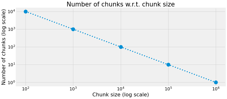
Number of chunks
n_chunks = [int(1000000 / c) for c in chunksizes]
plt.figure(figsize=(14, 6))
_ = plt.loglog(chunksizes, n_chunks, marker="o", markersize=15, linestyle=":")
ax = plt.gca()
_ = ax.set(
    title="Number of chunks w.r.t. chunk size",
    xlabel="Chunk size (log scale)",
    ylabel="Number of chunks (log scale)",
)
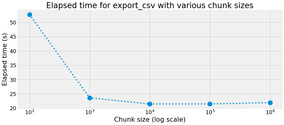
Elapsed time
timings = []
for chunksize in chunksizes:
    start = perf_counter()
    export_csv(chunksize=chunksize)
    end = perf_counter()
    elapsed_time = end - start
    timings.append(elapsed_time)
for chunksize, timing in zip(chunksizes, timings):
    print(f"chunk size : {chunksize:8d} rows, elapsed time : {timing:8.3f} s")
chunk size :      100 rows, elapsed time :   52.745 s
chunk size :     1000 rows, elapsed time :   23.624 s
chunk size :    10000 rows, elapsed time :   21.460 s
chunk size :   100000 rows, elapsed time :   21.470 s
chunk size :  1000000 rows, elapsed time :   21.929 s
plt.figure(figsize=(14, 6))
_ = plt.semilogx(chunksizes, timings, marker="o", markersize=15, linestyle=":")
ax = plt.gca()
_ = ax.set(
    title="Elapsed time for export_csv with various chunk sizes",
    xlabel="Chunk size (log scale)",
    ylabel="Elapsed time (s)",
)
Maximum memory usage
We compute the maximum memory usage using the memory_profiler package.
Warning: we noticed that the results were different when measuring the maximum memory within the JupyterLab notebook or within the console, the former being significantly larger. So we use a Python script export_csv_script.py to call the memory profiler for each chunk size, in the following way:
mem_usage = memory_usage(export_csv)
max_mem_usage = max(mem_usage)
print(f"max mem usage : {max_mem_usage}")
And call the script with the Python interpreter:
python export_csv_script.py
Here are the resulting measures:
max_mem_usage = [None] * 5
max_mem_usage[0] = 114.28515625
max_mem_usage[1] = 116.50390625
max_mem_usage[2] = 145.2265625
max_mem_usage[3] = 424.8359375
max_mem_usage[4] = 2111.64453125
for chunksize, max_mem in zip(chunksizes, max_mem_usage):
    print(f"chunk size : {chunksize:8d} rows, max memory usage : {max_mem:8.3f} MB")
chunk size :      100 rows, max memory usage :  114.285 MB
chunk size :     1000 rows, max memory usage :  116.504 MB
chunk size :    10000 rows, max memory usage :  145.227 MB
chunk size :   100000 rows, max memory usage :  424.836 MB
chunk size :  1000000 rows, max memory usage : 2111.645 MB
plt.figure(figsize=(14, 6))
_ = plt.semilogx(chunksizes, max_mem_usage, marker="o", markersize=15, linestyle=":")
ax = plt.gca()
_ = ax.set(
    title="Maximum memory usage for export_csv with various chunk sizes",
    xlabel="Chunk size (log scale)",
    ylabel="Maximum memory usage (MB)",
)
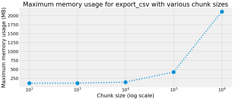
We can observe that in our case, an optimal chunk size is 10000 with an elapsed time of 21.460 s and a max memory usage of 145.227 MB.
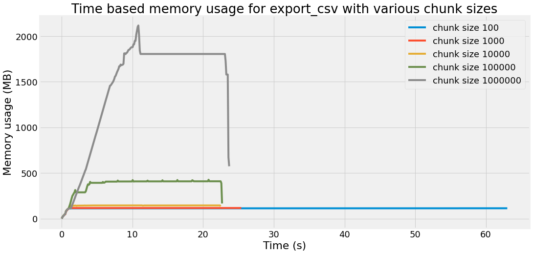
Time based memory usage
In this last section, we want to plot the temporal evolution of the memory usage, for each chunk size. In order to that, we use the memory_profiler package again, but from the command line:
mprof run export_csv_script.py
export_csv_script.py is a simple Python script calling the above export_csv function. Calling mprof run generates a mprofile_*.dat text file, that we open with Pandas read_csv().
dat_files = [f"mprofile_{chunksize}.dat" for chunksize in chunksizes]
dat_files
['mprofile_100.dat',
 'mprofile_1000.dat',
 'mprofile_10000.dat',
 'mprofile_100000.dat',
 'mprofile_1000000.dat']
def load_dat_file(fp):
    df = pd.read_csv(
        fp,
        sep=" ",
        skiprows=1,
        usecols=[1, 2],
        header=None,
        names=["memory_MB", "time_s"],
    )
    df["time_s"] = df["time_s"] - df["time_s"].values[0]
    return df
mem_profiles = []
for dat_file in dat_files:
    df = load_dat_file(dat_file)
    mem_profiles.append(df)
ax = mem_profiles[0].plot(
    x="time_s", y="memory_MB", label="chunk size 100", figsize=(16, 8)
)
ax = mem_profiles[1].plot(x="time_s", y="memory_MB", label="chunk size 1000", ax=ax)
ax = mem_profiles[2].plot(x="time_s", y="memory_MB", label="chunk size 10000", ax=ax)
ax = mem_profiles[3].plot(x="time_s", y="memory_MB", label="chunk size 100000", ax=ax)
ax = mem_profiles[4].plot(x="time_s", y="memory_MB", label="chunk size 1000000", ax=ax)
ax = plt.gca()
_ = ax.set(
    title="Time based memory usage for export_csv with various chunk sizes",
    xlabel="Time (s)",
    ylabel="Memory usage (MB)",
)