Trying DuckDB with Discogs data

This notebook is a small example of using DuckDB with the Python API.

What is DuckDB?

DuckDB is an in-process SQL OLAP Database Management System

It is a relational DBMS that supports SQL. OLAP stands for Online analytical processing, generally associated with complex queries, scanning a lot of data in order to generate some reports, as opposed to processing transactions. DuckDB is speeding up the data analysis process when dealing with rather large datasets. A key factor of this efficiency is the columnar-vectorized query execution engine. In-process means that DuckDB does not follow the client-server model and runs entirely within the host process.

DuckDB is released under a MIT License. How can you install DuckDB with the Python API? Well it is as simple as:

pip install duckdb

Voilà!

Discogs_Logo

What is Discogs? Here is a description from wikipedia:

Discogs is a website and crowdsourced database of information about audio recordings, including commercial releases, promotional releases, and bootleg or off-label releases.

Monthly dumps of Discogs data (Release, Artist, Label, and Master Release data) can be downloaded from their website, as compressed XML files. We used the nifty tool discogs-xml2db to convert the XML files into CSV files, that we are going to load into DuckDB. We also used it to load the same data into PostgreSQL in order to later measure and compare the execution time of a query.

In the following notebook, we are going to create a database with the following selection of tables (over 25+ available tables):

SELECTED_TABLE_NAMES = [  # Selection of tables to import into the DB
    "artist",
    "artist_alias",
    "artist_namevariation",
    "release",
    "release_genre",
    "release_artist",
]

Let’s start with the Python imports.

Imports

import glob
import os
import urllib
from time import perf_counter

import duckdb
import pandas as pd
import pyarrow.parquet as pq
from sqlalchemy import create_engine

Package versions:

Python          : 3.9.13 
duckdb          : 0.4.0
pyarrow         : 8.0.0
JupyterLab      : 3.4.3
Pandas          : 1.4.3

We also import some Jupyter extensions, so that we can create some SQL cells later:

%load_ext sql
%config SqlMagic.autopandas = True
%config SqlMagic.feedback = False
%config SqlMagic.displaycon = False

Data Loading

In order to batch import the data into DuckDB, we need some CSV or Parquet files. Here we have 6 CSV files, corresponding to the tables SELECTED_TABLE_NAMES from the Discogs database:

CSV_FILES = "/home/francois/Data/Disk_1/discogs_data/*.csv"

# list the CSV files located in the data directory
csv_file_paths = glob.glob(CSV_FILES)
csv_file_paths.sort()

# look for the CSV files corresponding to the selected tables
tables = []
for csv_file_path in csv_file_paths:
    csv_file_name = os.path.basename(csv_file_path)
    table_name = os.path.splitext(csv_file_name)[0]
    if table_name in SELECTED_TABLE_NAMES:
        tables.append((table_name, csv_file_path))
        file_size = os.path.getsize(csv_file_path) / 1000000.0
        print(f"Table {table_name:20s} - CSV file size : {file_size:8.2f} MB")

Table artist               - CSV file size :   580.77 MB
Table artist_alias         - CSV file size :   105.62 MB
Table artist_namevariation - CSV file size :    93.16 MB
Table release              - CSV file size :  2540.58 MB
Table release_artist       - CSV file size :  3973.41 MB
Table release_genre        - CSV file size :   369.94 MB

First we need to connect to the DuckDB database, specifying a file path:

conn = duckdb.connect(db_path)

If the database file does not already exists, it is created. The data is then loaded from the CSV files into the database, for example using a CREATE TABLE table_name AS SELECT * FROM 'csv_file_path' command. The database is saved into disk as a DuckDB file. In the present case, data loading takes around 5 minutes the first time:

CREATE TABLE artist AS SELECT * FROM '/home/francois/Data/Disk_1/discogs_data/artist.csv' - Elapsed time:   8.33 s
CREATE TABLE artist_alias AS SELECT * FROM '/home/francois/Data/Disk_1/discogs_data/artist_alias.csv' - Elapsed time:   8.35 s
CREATE TABLE artist_namevariation AS SELECT * FROM '/home/francois/Data/Disk_1/discogs_data/artist_namevariation.csv' - Elapsed time:   3.85 s
CREATE TABLE release AS SELECT * FROM '/home/francois/Data/Disk_1/discogs_data/release.csv' - Elapsed time:  38.06 s
CREATE TABLE release_artist AS SELECT * FROM '/home/francois/Data/Disk_1/discogs_data/release_artist.csv' - Elapsed time: 103.13 s
CREATE TABLE release_genre AS SELECT * FROM '/home/francois/Data/Disk_1/discogs_data/release_genre.csv' - Elapsed time: 138.63 s
CPU times: user 4min 47s, sys: 15.9 s, total: 5min 3s
Wall time: 5min

Two files are actually created by DuckDB:

DiscogsDB : 6.5GB
DiscogsDB.wal : 319 MB The .wal file a checkpoint file. It is actually removed when closing the connection, and not created when connecting to the database in read_only mode.

Subsequent connections only take a fraction of a second.

db_path = "/home/francois/Data/Disk_1/discogs_data/DiscogsDB"
db_exists = os.path.isfile(db_path)
db_exists

True

In the present case, the database has already been created, so we just connect to it in read-only mode. From the documentation:

If the database file does not exist, it will be created (the file extension may be .db, .duckdb, or anything else). The special value :memory: (the default) can be used to create an in-memory database. Note that for an in-memory database no data is persisted to disk (i.e. all data is lost when you exit the Python process). If you would like to connect to an existing database in read-only mode, you can set the read_only flag to True. Read-only mode is required if multiple Python processes want to access the same database file at the same time.

%%time
if not db_exists:

    conn = duckdb.connect(db_path, read_only=False)

    # load the CSV files and create the tables
    for table_name, csv_file_path in tables:
        query = f"""CREATE TABLE {table_name} AS SELECT * FROM '{csv_file_path}'"""
        start = perf_counter()
        conn.execute(query)
        elapsed_time_s = perf_counter() - start
        print(f"{query} - Elapsed time: {elapsed_time_s:6.2f} s")

else:

    conn = duckdb.connect(db_path, read_only=True)

CPU times: user 687 ms, sys: 187 ms, total: 873 ms
Wall time: 869 ms

Querying

Let’s test if the connection is working, by executing a query with the execute() method:

query = "SELECT COUNT(*) FROM artist"
conn.execute(query)
conn.fetchone()

(8107524,)

Seems to be OK!

Pandas

We can use the .df() method if we want the query execution to return a Pandas dataframe:

query = "SELECT * FROM artist LIMIT 5"
df = conn.execute(query).df()
df

	id	name	realname	profile	data_quality
0	1	The Persuader	Jesper Dahlbäck	NaN	Needs Vote
1	2	Mr. James Barth & A.D.	Cari Lekebusch & Alexi Delano	NaN	Correct
2	3	Josh Wink	Joshua Winkelman	After forming [l=Ovum Recordings] as an indepe...	Needs Vote
3	4	Johannes Heil	Johannes Heil	Electronic music producer, musician and live p...	Needs Vote
4	5	Heiko Laux	Heiko Laux	German DJ and producer based in Berlin. He is ...	Needs Vote

We could also create a table from a dataframe, if not in read_only mode, or query the dataframe in SQL:

query = "SELECT COUNT(*) FROM df"
conn.execute(query).fetchone()

(5,)

Arrow

We can export the result of a query as a PyArrow table:

query = "SELECT * FROM artist LIMIT 1000"
tabl = conn.execute(query).arrow()

type(tabl)

pyarrow.lib.Table

And also query this arrow table:

query = "SELECT COUNT(*) FROM tabl"
conn.execute(query).fetchone()

(1000,)

JupyterLab

We can also create some SQL cells directly using the DuckDB Python client. First we need to connect:

%sql duckdb:///{db_path}

Then we can create SQL cells starting with the %sql magic command:

%sql SELECT COUNT(*) FROM artist

	count_star()
0	8107524

What if we want a SQL cell to return a Pandas dataframe? We can assign the result of query to a dataframe using the << operator.

%sql df << SELECT * FROM release_artist LIMIT 3

Returning data to local variable df

df

	release_id	artist_id	artist_name	...	role	tracks
0	1	1	The Persuader	...	None	None
1	1	507025	George Cutmaster General	...	Lacquer Cut By	None
2	1	239	Jesper Dahlbäck	...	Written-By [All Tracks By]	None

%sql SELECT * FROM df WHERE artist_name = 'The Persuader'

	release_id	artist_id	artist_name	...	role	tracks
0	1	1	The Persuader	...	None	None

Export

We can export the result of a SQL query into a CSV or a Parquet file.

CSV export

A COPY statement can bu used to export the result of a query as a CSV file:

csv_file_path = "./artist.csv"

%sql COPY (SELECT * FROM artist LIMIT 1000) TO '{csv_file}' WITH (HEADER 1, DELIMITER ',');

	Count
0	1000

Parquet export

parquet_file_path = "./artist.parquet"

%sql COPY (SELECT * FROM artist LIMIT 1000) TO '{parquet_file_path}' (FORMAT PARQUET);

	Count
0	1000

table = pq.read_table(parquet_file_path)

table.shape

(1000, 5)

The Parquet file can also be queried directly:

%sql SELECT * FROM read_parquet('{parquet_file_path}') LIMIT 5;

	id	name	realname	profile	data_quality
0	1	The Persuader	Jesper Dahlbäck	None	Needs Vote
1	2	Mr. James Barth & A.D.	Cari Lekebusch & Alexi Delano	None	Correct
2	3	Josh Wink	Joshua Winkelman	After forming [l=Ovum Recordings] as an indepe...	Needs Vote
3	4	Johannes Heil	Johannes Heil	Electronic music producer, musician and live p...	Needs Vote
4	5	Heiko Laux	Heiko Laux	German DJ and producer based in Berlin. He is ...	Needs Vote

As explained in the documentation:

The Parquet file will be processed in parallel. Filters will be automatically pushed down into the Parquet scan, and only the relevant columns will be read automatically.

There are many many more useful features available with DuckDB and we refer to the documentation for an overview of all what can be done with DuckDB. Now let’s focus on a simple test case.

A More complex query

Now we are going to create a little more complex query. We want to compute the number of releases per year and per music genre. So we only need to use 2 distinct tables: release and release_genre. One of the issues is that the year_released column from the contains a string entered by the Discogs contributors, that may vary in its form, but usually looks like yyyy-mm-dd. In order to get the release year, we are going to take the first 4 characters from the year_released field and assume it’s a numeric year.

query = """SELECT se.year_released,
       se.genre,
       Count(*) AS release_count
FROM   (SELECT Substr(re.released, 1, 4) AS YEAR_RELEASED,
               re.id,
               re_g.genre
        FROM   release AS re
               LEFT JOIN release_genre AS re_g
                      ON re.id = re_g.release_id
        WHERE  re.released IS NOT NULL
               AND re.released NOT IN ( '?' )) AS se
GROUP  BY se.year_released,
          se.genre
ORDER  BY release_count DESC"""

DuckDB

start = perf_counter()
df1 = conn.execute(query).df()
elapsed_time_s_1 = perf_counter() - start
print(f"Elapsed time: {elapsed_time_s_1:6.2f} s")
df1.head()

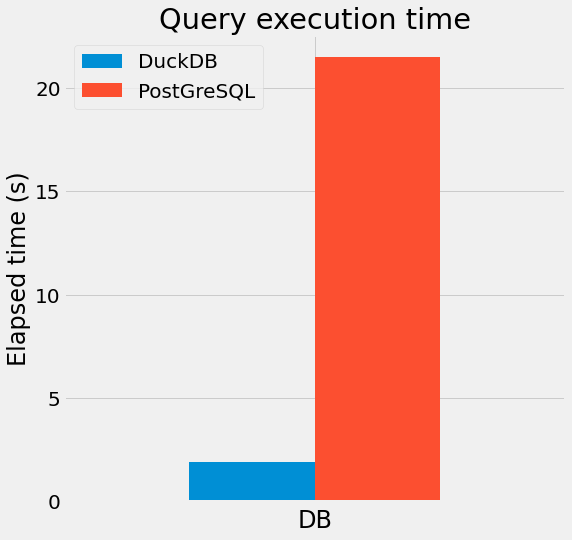
Elapsed time:   1.81 s

	YEAR_RELEASED	genre	release_count
0	2020	Electronic	162166
1	2018	Electronic	156421
2	2019	Electronic	152393
3	2017	Electronic	151043
4	2016	Electronic	148127

df1.shape

(1647, 3)

PostgreSQL

PostgreSQL client and server are installed on the same computer as DuckDB.

PG_USERNAME = "discogs_user"
PG_PASSWORD = "****"
PG_SERVER = "localhost"
PG_PORT = 5432
PG_DATABASE = "discogsdb"
CONNECT_STRING = (
    f"postgresql+psycopg2://{PG_USERNAME}:"
    + f"{urllib.parse.quote_plus(PG_PASSWORD)}@{PG_SERVER}:{PG_PORT}/{PG_DATABASE}"
)

engine = create_engine(CONNECT_STRING)

start = perf_counter()
df2 = pd.read_sql(query, engine)
elapsed_time_s_2 = perf_counter() - start
print(f"Elapsed time: {elapsed_time_s_2:6.2f} s")
df2.head()

Elapsed time:  21.51 s

	year_released	genre	release_count
0	2020	Electronic	162166
1	2018	Electronic	156421
2	2019	Electronic	152393
3	2017	Electronic	151043
4	2016	Electronic	148127

df2.shape

(1647, 3)

df = pd.DataFrame(
    data={"DuckDB": [elapsed_time_s_1], "PostGreSQL": [elapsed_time_s_2]},
    index=[""],
)
ax = df.plot.bar(figsize=(6, 6))
_ = ax.set(title="Query execution time", xlabel="DB", ylabel="Elapsed time (s)")

Query execution time

So the same query on the same computer is executed about 10 times faster with DuckDB than with PostgreSQL (both DB with default settings).

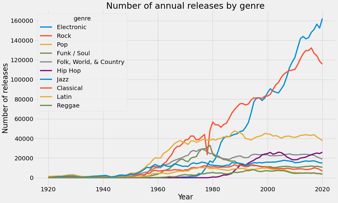
To conclude this post, let’s plot the result of the previous query with Pandas/Matplotlib.

Evolution of the 10 most popular genres ever

The first job is to filter out ambiguous entries such as 197, 197?, 70's and convert the year variable to int … Then we pivot the table in order to have each genre in a distinct column. We select years between 1940 and 2020 (data might be missing for the recent releases, in 2021 and 2022, because it has not been entered into the DB yet).

df1 = df1[df1.YEAR_RELEASED.str.isnumeric() & (df1.YEAR_RELEASED.str.len() == 4)].copy(
    deep=True
)
df1.YEAR_RELEASED = df1.YEAR_RELEASED.astype(int)
df1.rename(columns={"YEAR_RELEASED": "year"}, inplace=True)
df1 = df1.pivot_table(index="year", columns="genre", values="release_count")
df1 = df1.fillna(0)
df1 = df1.astype(int)
df1 = df1[(df1.index >= 1940) & (df1.index <= 2020)]
df1.sort_index(inplace=True)
order_max = df1.max().sort_values(ascending=False).index
df1 = df1[order_max[:10]]
df1.tail(3)

genre	Electronic	Rock	Pop	...	Latin	Reggae
year
2018	156421	124208	41438	...	4106	4321
2019	152393	118760	39830	...	4039	4189
2020	162166	115612	37814	...	3280	3813

ax = df1.plot(figsize=(16, 10), legend=True, grid=True)
_ = ax.set(
    title=f"Number of annual releases by genre",
    xlabel="Year",
    ylabel="Number of releases",
)

Number of annual releases by genre

Kind of sad to see Jazz so low.

Close the DuckDB connection

%%time
conn.close()

CPU times: user 26.3 ms, sys: 4.55 ms, total: 30.8 ms
Wall time: 29.1 ms