Euler’s number and the uniform sum distribution

Last year I stumbled upon this tweet from @fermatslibrary [1]:

I find it a little bit intriguing for Euler’s number $e$ to appear here! But actually, it is not uncommon to encounter $e$ in probability theory, as explained by Stefanie Reichert in the short article e is everywhere [2].

Let’s derive mathematically the above statement and perform random experiments in Python (and Numba, to speed up the computations).

A First Python experiment

We start with a very simple experiment to evaluate the average number of random numbers between 0 and 1 required to go over 1 when summing them:

%%time
import numpy as np


def eval_N():
    """N is the number of random samples drawn from a uniform
    distribution over [0, 1) that we need to pick so that their
    sum is strictly greater than 1.

    Returns:
        float: The value of N.
    """
    s, N = 0.0, 0
    while s <= 1.0:
        s += np.random.rand()
        N += 1
    return N


RS = 124  # random seed
np.random.seed(RS)
n_eval = 1_000_000  # number of evaluations
m = 0.0  # m is the average value of n
for i in range(n_eval):
    m += eval_N()
m /= n_eval
print(f"m = {m:6.4f}")

m = 2.7179
CPU times: user 1.71 s, sys: 326 ms, total: 2.03 s
Wall time: 1.51 s

Indeed, not so far from $e$!

np.e

2.718281828459045

Before we dive into some probability distributions, let’s import all the other packages required for this notebook.

from functools import partial
from math import comb, factorial

import matplotlib
import matplotlib.pyplot as plt
import pandas as pd
from numba import jit, njit, prange

FS = (15, 8)  # figure size
CMAP = "plasma"  # color map

Mathematical formulation

First of all, we consider some independent and identically distributed (i.i.d) random variables $ \left\{ U_k \right\}_{ k \geq 1}$, each having standard uniform distribution $\mathbf{U}(0,1)$. For $x > 0$, we define $N(x)$ as the following:

\[N(x) \equiv \min \left\{ n \in \mathbb{N}^* \; s.t. \; \sum_{k=1}^n U_k > x \right\}\]

We are actually interested in the expected value of $N$:

\[m(x) \equiv E \left[ N(x) \right]\]

The above statement in Fermat’s Library’s tweet can be expressed like this: $m(1)$ is equal to $e$.

First of all, let’s look at the distribution of $\sum_{k=1}^n U_k > x$, which is referred to as the Irwin-Hall distribution.

The Irwin-Hall distribution

The Irwin-Hall distribution is the continuous probability distribution of the sum of $n$ i.i.d random variables, each having standard uniform distribution $\mathbf{U}(0,1)$:

\[X_n = \sum_{k=1}^n U_k\]

It is also called the uniform sum distribution. $X_n$ has a continuous distribution with support $[0, n]$ for $n \in \mathbb{N}^* $.

Cumulative ditribution function of Irwin-Wall distribution

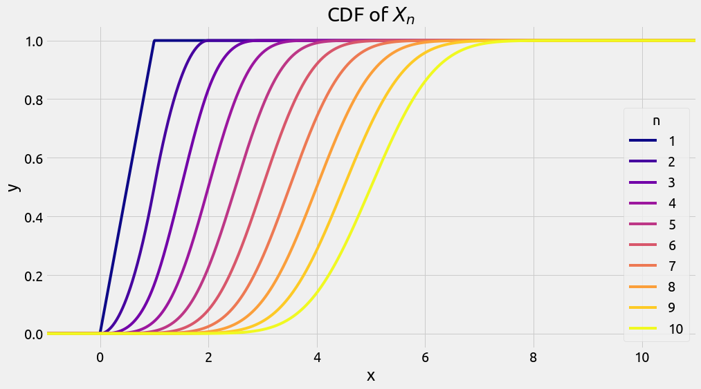
For $x > 0$ and $n \in \mathbb{N}^* $, the Cumulative Distribution Function (CDF) of $X_n$ is the following one:

\[F_{X_n}(x)= \frac{1}{n!} \sum_{k=0}^{\lfloor x \rfloor} (-1)^k { {n}\choose{k} } (x-k)^n\]

See [3] for a complete derivation of this formula (not trivial). The CDF corresponds to the probability that the variable, $X_n$ in our case, takes on a value less than or equal to $x$:

\[P \left[ X_n \leq x \right] = F_{X_n}(x)\]

Let’s write a function cdf_th to compute this CDF:

def cdf_th(x, n=2):
    """Analytical cumulative distribution of the Irwin-Wall distribution.

    Args:
        x (float): input of the cumulative distribution function.
        n (int): number of uniform random variables in the summation.

    Returns:
        float: The function value at x.
    """
    if x <= 0.0:
        return 0.0
    elif x >= n:
        return 1.0
    else:
        x_floor = int(np.floor(x))
        cdf = 0
        for k in range(x_floor + 1):
            cdf += np.power(-1.0, k) * comb(n, k) * np.power(x - k, n)
        cdf /= factorial(n)
        return cdf

We can evaluate and plot this CDF for various values of $n$:

x = np.linspace(-1, 11, 1000)
cdf_th_df = pd.DataFrame(data={"x": x})
for n in range(1, 11):
    y = list(map(partial(cdf_th, n=n), x))
    cdf_th_df[str(n)] = y

ax = cdf_th_df.plot(x="x", figsize=FS, grid=True, cmap=CMAP)
_ = ax.legend(title="n")
_ = ax.set(title="CDF of $X_n$", xlabel="x", ylabel="y")
_ = ax.set_xlim(-1, 11)

CDF of $X_n$$

But we can also try to approach this analytical CDF with some observations, adding scalar drawn from the uniform distribution in the interval [0, 1).

The Empirical CDF

This part is inspired by a great blog post [4] by Keith Goldfeld, with some R code. We are going to use np.random.rand() to build an empirical CDF.

def cdf_emp(n=5, s=100_000, rs=124):
    """Empirical cumulative distribution of the Irwin-Wall distribution.

    Args:
        n (int): number of uniform random variables in the summation.
        s (int): number of samples used to evaluate the distribution.
        rs (int): random seed.

    Returns:
        (float, float): the x and y data points of the approached CDF.
    """
    arr = np.empty(s, dtype=np.float64)
    np.random.seed(rs)
    for i in prange(s):
        c = 0.0
        for k in range(n):
            c += np.random.rand()
        arr[i] = c
    x = np.sort(arr)
    y = np.arange(s) / np.float64(s)
    return x, y

%%time
x, y = cdf_emp(n=10, rs=RS)

CPU times: user 461 ms, sys: 3.7 ms, total: 465 ms
Wall time: 463 ms

cmap = matplotlib.cm.get_cmap(CMAP)
ax = cdf_th_df.plot(
    x="x", y="10", figsize=FS, alpha=0.6, label="Theoretical", c=cmap(0)
)
_ = ax.scatter(x, y, label="Empirical", alpha=0.6, s=50, color=cmap(0.8))
_ = ax.legend()
_ = ax.set(title="Theoretical and empirical CDF of $X_{10}$", xlabel="x", ylabel="y")

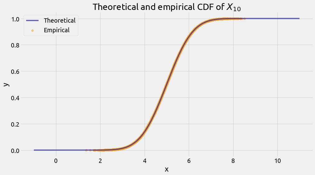
$Theoretical and empirical CDF of $X_{10}$$

Actually we can do that for several values of $n$, as we did precedently with the analytical CDF:

cdf_emp_df = pd.DataFrame()
for n in range(1, 11):
    x, y = cdf_emp(n=n)
    cdf_emp_df["x_" + str(n)] = x
    cdf_emp_df["y_" + str(n)] = y

ax = cdf_emp_df.plot(x="x_1", y="y_1", figsize=FS, label="1", c=cmap(0))
for n in range(2, 11):
    ax = cdf_emp_df.plot(
        x="x_" + str(n), y="y_" + str(n), ax=ax, label=str(n), c=cmap((n - 1) / 9)
    )
_ = ax.legend(title="n")
_ = ax.set(
    title="Empirical CDF of $X_n$",
    xlabel="x",
    ylabel="y",
)
_ = ax.set_xlim(-1, 11)

Empirical CDF of $X_n$

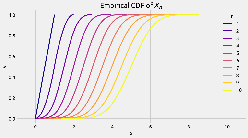
Now that we went over the CDF of the Irwin-Wall distribution, we can proceed to derive a formula for $m(x)$.

Mathematical derivation of $m(x)$

For $n \in \mathbb{N}^* $, we have:

\[\begin{align*} P \left[ N(x) = n \right] &= P \left[ (X_{n-1} \leq x) \; \& \; (X_n > x) \right] \\ &= P\left[ (X_n > x) \; | \; (X_{n-1} \leq x) \right] P\left[ X_{n-1} \leq x \right] \\ &= \left( 1 - P\left[ (X_n \leq x) \; | \; (X_{n-1} \leq x) \right] \right) P\left[ X_{n-1} \leq x \right] \\ &= \left( 1 - \frac{P\left[ (X_{n-1} \leq x) \; \& \; (X_n \leq x) \right]}{P\left[ X_{n-1} \leq x \right]} \right) P\left[ X_{n-1} \leq x \right] \\ &= \left( 1 - \frac{P\left[ X_n \leq x \right]}{P\left[ X_{n-1} \leq x \right]} \right) P\left[ X_{n-1} \leq x \right] \\ &= P\left[ X_{n-1} \leq x \right] - P\left[ X_n \leq x) \right] \end{align*}\]

A derivation for $x=1$ can be also found in the blog post [4] by Keith Goldfeld.

Because we know the CDF for $X_n$, and thus for $X_{n-1}$, we can write:

\[\begin{align*} P \left[ N(x) = n \right] &= F_{X_{n-1}}(x) - F_{X_n}(x) \\ &= \frac{1}{(n-1)!} \sum_{k=0}^{\lfloor x \rfloor} (-1)^k { {n-1}\choose{k} } (x-k)^{n-1} \\ &- \frac{1}{n!} \sum_{k=0}^{\lfloor x \rfloor} (-1)^k { {n}\choose{k} } (x-k)^{n} \\ &= \frac{1}{(n-1)!} \sum_{k=0}^{\lfloor x \rfloor} \frac{(-1)^k (x-k)^{n-1}}{n} { {n}\choose{k} } (n-x) \end{align*}\]

Also, we can observe that $P \left[ N(x) = n \right] = 0$ if $ n < \lceil x \rceil$. This is because:

\[\forall n \in \mathbb{N}^* , \; \sum_{k=1}^n U_k \leq n \; \Rightarrow \; N(x) \geq \lceil x \rceil\]

We can know derive a formula for $m(x)$:

\[\begin{align*} m(x) &= E\left[ N(x) \right] \\ &= \sum_{n=0}^{\infty} n P \left[ N(x) = n \right] \\ &= \sum_{n=\lceil x \rceil}^{\infty} \frac{n}{(n-1)!} \sum_{k=0}^{\lfloor x \rfloor} \frac{(-1)^k (x-k)^{n-1}}{n} { {n}\choose{k} } (n-x) \\ &= \sum_{n=\lceil x \rceil}^{\infty} n (n-x) \sum_{k=0}^{\lfloor x \rfloor} \frac{(-1)^k (x-k)^{n-1}}{k! (n-k)!} \end{align*}\]

So let’s find the exact value of $m(1)$ using the power series expansion $e^x = \sum_{n=0}^{\infty} \frac{x^n}{n!}$:

\[\begin{align*} m(1) &= \sum_{n=2}^{\infty} n (n-1) \sum_{k=0}^1 \frac{(-1)^k (1-k)^{n-1}}{k! (n-k)!} \\ &= \sum_{n=2}^{\infty} n (n-1) \left[ \frac{1}{n!} + 0 \right] \\ &= \sum_{n=2}^{\infty} \frac{1}{(n-2)!} = \sum_{n=0}^{\infty} \frac{1}{n!} = e \end{align*}\]

So we finally got our result:

\[m(1) = e\]

success

With a little bit longer derivation (this is why we are not going to display it here), we can show that:

\[m(2) = e^2 -e\]

Wolfram MathWorld’s web page about the Uniform Sum Distribution [5], also lists the values of $m(x)$ for the next integer values of $x$:

\[\begin{align*} m(3) &= \frac{1}{2} \left( 2 e^3 -4 e^2 + e\right) \\ m(4) &= \frac{1}{6} \left( 6 e^4 -18 e^3 + 12 e^2 - e\right) \\ m(5) &= \frac{1}{24} \left( 24 e^5 - 96 e^4 + 108 e^3 - 32 e^2 + e\right) \\ \end{align*}\]

We can write a function that approaches the $m(x)$ formula. This is an approximation because we try to compute an infinite sum with a finite loop.

def analytical_m(x, n_max=150):
    """Approximation of the analytical formula for m(x).

    Args:
        x (float): input value of m.
        n_max (int): end of loop.

    Returns:
        float: the computed value for m(x).
    """
    x = float(x)
    m = 0.0
    for n in range(int(np.ceil(x)), n_max):
        s = 0.0
        for k in range(int(np.ceil(x))):
            s += (
                np.power(-1, k)
                * np.power(x - k, n - 1)
                / (np.math.factorial(k) * np.math.factorial(n - k))
            )
        m += n * (n - x) * s
    return m

Comparing the approximated analytical values of $m(x)$ with the exact values, we get:

m = {}
m[1] = np.e
m[2] = np.exp(2) - np.e
m[3] = 0.5 * (2 * np.exp(3) - 4 * np.exp(2) + np.e)
m[4] = (6 * np.exp(4) - 18 * np.exp(3) + 12 * np.exp(2) - np.e) / 6.0
m[5] = (
    24 * np.exp(5) - 96 * np.exp(4) + 108 * np.exp(3) - 32 * np.exp(2) + np.e
) / 24.0

for x in range(1, 6):
    print(
        f"x={x}, m({x}) = {m[x]:12.10f}, approximated m({x}) = {analytical_m(x):12.10f}"
    )

x=1, m(1) = 2.7182818285, approximated m(1) = 2.7182818285
x=2, m(2) = 4.6707742705, approximated m(2) = 4.6707742705
x=3, m(3) = 6.6665656396, approximated m(3) = 6.6665656396
x=4, m(4) = 8.6666044900, approximated m(4) = 8.6666044900
x=5, m(5) = 10.6666620686, approximated m(5) = 10.6666620686

Quite close! Now that that we are rather confident about the accuracy of the approximation of $m(x)$, we may evaluate and plot it on a discretized segment:

x_max = 6
x = np.linspace(0.001, x_max, 500)
m_th_df = pd.DataFrame(data={"x": x})
y = list(map(analytical_m, x))
m_th_df["m(x)"] = y

ax = m_th_df.plot(
    x="x", y="m(x)", figsize=FS, grid=True, cmap=CMAP, legend=True, label="Approximated"
)
_ = ax.set(title="m(x)", xlabel="x", ylabel="y")
_ = ax.set_xlim(0, x_max)
points = [(1, m[1]), (2, m[2]), (3, m[3]), (4, m[4]), (5, m[5])]
label = "Exact value"
for point in points:
    _ = plt.plot(
        point[0],
        point[1],
        marker="o",
        alpha=0.5,
        markersize=20,
        markerfacecolor="y",
        label=label,
    )
    label = None
_ = ax.legend()

m(x)

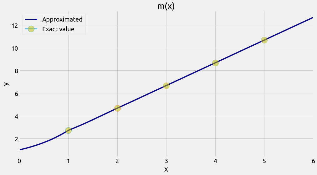
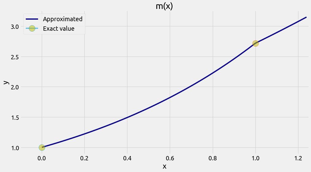
It kind of looks like it becomes a straight line for larger values of $x$. Also, it is easy to show what’s the limit of $m(x)$ when $x$ goes to 0:

\[\begin{align*} \lim_{x \to 0⁺} m(x) &= \lim_{x \to 0⁺} \sum_{n=1}^{\infty} \frac{(n-x) x^{n-1}}{(n-1)!} \\ &= \lim_{x \to 0⁺} e^x \\ &= 1 \end{align*}\]

It makes sense since a single random number is almost sure to be strictly larger than zero. Zooming toward the left part of $m(x)$, its shape is easier to see.

x_max = 1.25
ax = m_th_df.loc[m_th_df.x < x_max].plot(
    x="x", y="m(x)", figsize=FS, grid=True, cmap=CMAP, legend=True, label="Approximated"
)
_ = ax.set(title="m(x)", xlabel="x", ylabel="y")
_ = ax.set_xlim(-0.1, x_max)
_ = plt.plot(
    0,
    1,
    marker="o",
    alpha=0.5,
    markersize=20,
    markerfacecolor="y",
    label="Exact value",
)
_ = plt.plot(
    points[0][0],
    points[0][1],
    marker="o",
    alpha=0.5,
    markersize=20,
    markerfacecolor="y",
    label=None,
)
_ = ax.legend()

left part of m(x)

Computation of $m(x)$ with a Numba experiment

To finish this post, let’s come back to the first piece of code where we performed a random experiment to approximate $m(1)$. But this time we are going to do it more efficiently by:

using Numba to make the code faster
using a parallel loop
using a different random seed in each chunk of computed values (although I am not very sure it improves the result)

Note that it is OK to use np.random.rand() in some multi-threaded Numba code, as we can read in their documentation:

Since version 0.28.0, the generator is thread-safe and fork-safe. Each thread and each process will produce independent streams of random numbers.

We are using Numba version 0.55.2.

@njit(parallel=True)
def compute_m_with_numba(
    n: int = 1_000, x: float = 1.0, rs_init: int = 124, chunk_size: int = 100_000
):
    """Empirical evaluation of m(x) with Numba.

    Args:
        n (float): number of evaluations.
        x (float): input value of m.
        rs_init (int): initial random seed.
        chunk_size (int): number of evaluations perfomed with same random seed.

    Returns:
        float: the computed value for m(x).
    """
    # random seed
    rs = rs_init

    # number of chunks
    num_chunks = n // chunk_size + 1
    if n % chunk_size == 0:
        num_chunks -= 1

    n_min_tot = 0
    count_tot = 0
    r = n
    while r > 0:
        np.random.seed(rs)

        if r < chunk_size:
            n_loc = r
        else:
            n_loc = chunk_size

        for i in prange(n_loc):
            s = 0.0  # sum
            count = 0  # number of added uniform random variables
            while s <= x:
                s += np.random.rand()
                count += 1
            n_min_tot += count
        count_tot += n_loc

        r -= n_loc
        rs += 1  # change the random seed

    return n_min_tot / count_tot


n = 1_000
m_1_exper = compute_m_with_numba(n, x=1.0)
print(f"m(1) = {m_1_exper} approximated with {n} experiments (e={np.e})")

m(1) = 2.77 approximated with 1000 experiments (e=2.718281828459045)

Let’s perform a billion random evaluations.

%%time
n = 1_000_000_000
m_1_exper = compute_m_with_numba(n, x=1.0)
print(f"m(1) = {m_1_exper} approximated with {n} experiments (e={np.e})")

m(1) = 2.71828312 approximated with 1000000000 experiments (e=2.718281828459045)
CPU times: user 1min 6s, sys: 18.3 ms, total: 1min 7s
Wall time: 8.61 s

This takes about 8s on my 8 core CPU.

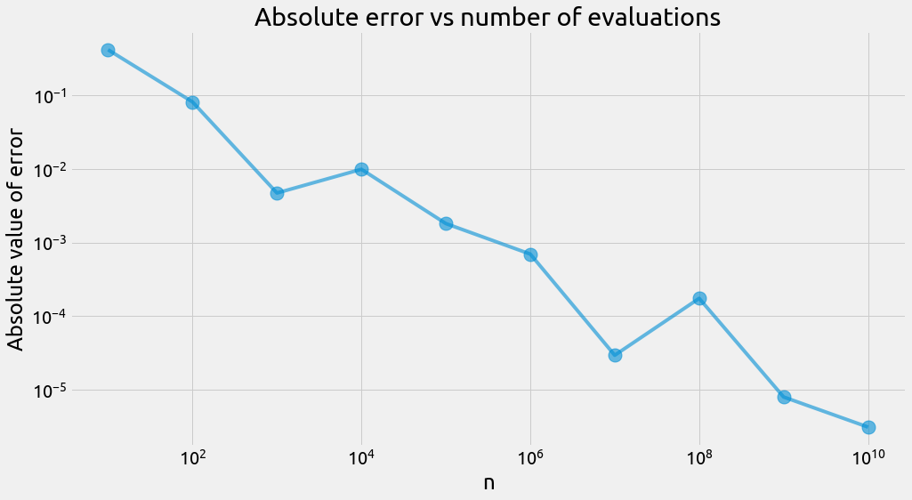
Now how does the absolute error evolve with the number of evaluations?

%%time
start = 1
end = 10
ns = [int(n) for n in np.logspace(start, end, num=end - start + 1)]
errors = []
for n in ns:
    errors.append(compute_m_with_numba(n) - np.e)
errors_df = pd.DataFrame(data={"n": ns, "error": errors})
errors_df["error_abs"] = errors_df["error"].abs()

CPU times: user 15min 49s, sys: 837 ms, total: 15min 49s
Wall time: 2min 9s

ax = errors_df.plot(
    x="n",
    y="error_abs",
    loglog=True,
    grid=True,
    figsize=FS,
    legend=False,
    style="o-",
    ms=15,
    alpha=0.6,
)
_ = ax.set(
    title="Absolute error vs number of evaluations",
    xlabel="n",
    ylabel="Absolute value of error",
)

Absolute error vs number of evaluations

References

[1] https://twitter.com/fermatslibrary/status/1388491536640487428?s=20
[2] Reichert, S. e is everywhere. Nat. Phys. 15, 982 (2019). https://doi.org/10.1038/s41567-019-0655-9
[3] Random Services https://www.randomservices.org/random/special/IrwinHall.html
[4] Keith Goldfeld - Using the uniform sum distribution to introduce probability
[5] Wolfram MathWorld - Uniform Sum Distribution