Forward and reverse star representation of a digraph

In this Python notebook, we are going to focus on a graph representation of directed graphs : the forward star representation (and its opposite, the reverse star). The motivation here is to access a network topology and associated data efficiently, without using a large amount of memory space. In many shortest path algorithms, one needs to quickly access the outgoing or incoming edges of the graph vertices, as well as the associated edge attributes. This is why the data structure used to represent the graph is very important regarding the efficiency of graph algorithms. Note that we only consider static graphs here, where the topology does not change.

Definitions

From wikipedia:

a directed graph (or digraph) is a graph that is made up of a set of vertices connected by directed edges, often called arcs.

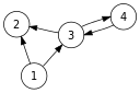
Credit: Wikimedia Commons

Here we indifferently use the terms edge, arc or link. Same thing with node or vertex. Also, we denote the two nodes of an arc as head and tail nodes, or target and source nodes, or from node and to node.

Let’s denote the directed graph $\mathcal{G} = \left( V, E \right) $, where $V$ and $E$ are the graph vertices and edges. The head vertices of the outgoing edges of vertex $v_i$:

\[E_i^+ = \left\{ j \in V \; s.t. \; (i,j)\in E\right\}\]

The tail vertices of the incoming edges of vertex $v_j$:

\[E_j^- = \left\{ i \in V \; s.t. \; (i,j)\in E\right\}\]

In the small example above, the incoming edges of vertex 3 are : (1, 3) and (4, 3). Its outgoing edges are : (3, 2) and (3, 4).

Imports

from collections import namedtuple

import networkx as nx
import numpy as np
import pandas as pd
from scipy.sparse import coo_array, csc_matrix, csr_matrix

A Small toy network

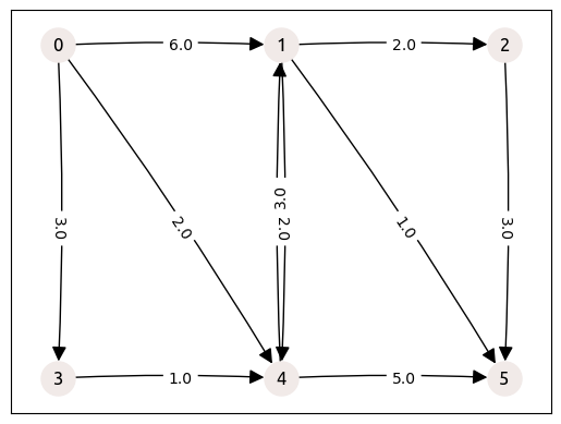
In order to describe the topology of a graph, we just need the edge table with tail node index, head node index and edge attributes. Here we use a Pandas dataframe to store this table. Let’s take the small example from Sheffi [1] with 10 edges:

tail_verts = np.array([1, 3, 0, 4, 1, 1, 0, 2, 0, 4], dtype=np.uint32)
head_verts = np.array([2, 4, 4, 5, 4, 5, 3, 5, 1, 1], dtype=np.uint32)
edge_weights = np.array([2, 1, 2, 5, 2, 1, 3, 3, 6, 3], dtype=np.float64)
edges_df = pd.DataFrame(
    data={"from_node": tail_verts, "to_node": head_verts, "weight": edge_weights}
)
edges_df.head(3)

	from_node	to_node	weight
0	1	2	2.0
1	3	4	1.0
2	0	4	2.0

vertex_count = edges_df[["from_node", "to_node"]].max().max() + 1
edge_count = len(edges_df)
print(f"vertex count : {vertex_count},  edge count : {edge_count}")

vertex count : 6,  edge count : 10

Note that this network only has only a single attribute per edge, weight, which is of float64 type. The node indices are of uint32 type, which is allowing us to deal with more than 4 billion nodes:

np.iinfo(np.uint32)

iinfo(min=0, max=4294967295, dtype=uint32)

We can load this network into NetworkX in order to plot it, in the following way:

G = nx.from_pandas_edgelist(
    edges_df,
    source="from_node",
    target="to_node",
    edge_attr="weight",
    create_using=nx.DiGraph,
)
type(G)

networkx.classes.digraph.DiGraph

pos = {
    0: (0, 1),
    1: (1, 1),
    2: (2, 1),
    3: (0, 0),
    4: (1, 0),
    5: (2, 0),
}  # here we assign some coordinates to each vertex
nx.draw_networkx(
    G,
    pos,
    arrowsize=20,
    node_color="#F1EAE8",
    node_size=500,
    font_family="ubuntu",
    connectionstyle="arc3,rad=-0.025",
)
labels = nx.get_edge_attributes(G, "weight")
_ = nx.draw_networkx_edge_labels(G, pos, edge_labels=labels, label_pos=0.45)

networkx

Sparse matrix formats

We can represent the graph as a Node-Node Adjacency Matrix with a sparse format.

Let’s start by describing the Node-Node Adjacency Matrix. If the graph does not have any parallel edge, it can be expressed as a (vertex_count x vertex_count) matrix, where rows correspond to tail nodes and columns to head nodes. The (i, j)-th entry equals 1 if $(i, j) \in E$, and 0 otherwise.

M = np.zeros((vertex_count, vertex_count), dtype=np.uint32)
M[edges_df["from_node"].values, edges_df["to_node"].values] = 1
M

array([[0, 1, 0, 1, 1, 0],
       [0, 0, 1, 0, 1, 1],
       [0, 0, 0, 0, 0, 1],
       [0, 0, 0, 0, 1, 0],
       [0, 1, 0, 0, 0, 1],
       [0, 0, 0, 0, 0, 0]], dtype=uint32)

Because this kind of matrix has a lot of zeros when dealing with sparse graphs, we only store the non-zero entries. The most simple sparse storage format is the COO matrix format, that we are going to see in the next sub-section.

Because we want to access some edge attributes, we do not store an array of ones as non-zeros, as it is described just above. Instead, we store the attributes. In the present example, the data vector is 1D as there is only a single edge attribute: weight. So here is the actual matrix that we want to represent with a sparse format:

M = np.zeros((vertex_count, vertex_count), dtype=np.float64)
M[edges_df["from_node"].values, edges_df["to_node"].values] = edges_df["weight"].values
M

array([[0., 6., 0., 3., 2., 0.],
       [0., 0., 2., 0., 2., 1.],
       [0., 0., 0., 0., 0., 3.],
       [0., 0., 0., 0., 1., 0.],
       [0., 3., 0., 0., 0., 5.],
       [0., 0., 0., 0., 0., 0.]])

COO format

Coordinate list (COO) stores a list of (row, column, value) tuples. It is also know as triplet format. Here, we access to the COO data column-wise:

coo_row = edges_df["from_node"].values
coo_col = edges_df["to_node"].values
coo_val = edges_df["weight"].values

Let’s create a SciPy sparse matrix in COOrdinate format with scipy.sparse.coo_matrix in order to check our computations later .

sp_coo = coo_array(
    (coo_val, (coo_row, coo_col)),
    dtype=np.float64,
    shape=(vertex_count, vertex_count),
)

assert np.allclose(coo_row, sp_coo.row)
assert np.allclose(coo_col, sp_coo.col)
assert np.allclose(coo_val, sp_coo.data)
type(sp_coo)

scipy.sparse._arrays.coo_array

Now we are going to use another very common sparse format, called Compressed Sparse Row (CSR) or Compressed Row Storage (CRS). This storage it directly related to the forward star representation of a graph.

CSR format

Here is a detailed description from netlib:

The Compressed Row and Column Storage formats are the most general: they make absolutely no assumptions about the sparsity structure of the matrix, and they don’t store any unnecessary elements. On the other hand, they are not very efficient, needing an indirect addressing step for every single scalar operation in a matrix-vector product or preconditioner solve.

The Compressed Row Storage (CRS) format puts the subsequent nonzeros of the matrix rows in contiguous memory locations. Assuming we have a nonsymmetric sparse matrix, we create vectors: one for floating-point numbers (val), and the other two for integers (col_ind, row_ptr). The val vector stores the values of the nonzero elements of the matrix, as they are traversed in a row-wise fashion. The col_ind vector stores the column indexes of the elements in the val vector.

That is, if val[k] = a[i,j] then col_ind[k]=j. The row_ptr vector stores the locations in the val vector that start a row, that is, if val[k] = a[i,j] then row_ptr[i] <= k <= row_ptr[i+1]. By convention, we define row_ptr[n+1] = nnz + 1, where nnz is the number of nonzeros in the matrix A. The storage savings for this approach is significant. Instead of storing n² elements, we need only 2 nnz + n + 1 storage locations.

Let’s see how to convert from COO to CSR sparse formats in Python.

Convert COO to CRS

One requirement is that the edge list in COO format must be sorted in an ascending way by the tail node index. In the following, we also sort secondly by the head node index in order to match the result from the SciPy.sparse library, however this is not required. This implies that for each vertex, the resulting list of outgoing edges will also be sorted, by the head vertex index.

edges_df.sort_values(by=["from_node", "to_node"], axis=0, ascending=True, inplace=True)
coo_row = edges_df["from_node"].values
coo_col = edges_df["to_node"].values
coo_val = edges_df["weight"].values

We start by creating the NumPy arrays for storing the CSR representation. vertex_count is the dimension of the matrix, while edge_count is the number of non-zero elements, resulting to 2 edge_count + vertex_count + 1 storage locations, as seen above:

csr_indptr = np.zeros(vertex_count + 1, dtype=np.uint32)
csr_indices = np.zeros(edge_count, dtype=np.uint32)
csr_data = np.zeros(edge_count, dtype=np.float64)

for i in range(edge_count):
    csr_indptr[coo_row[i] + 1] += 1
    csr_indices[i] = coo_col[i]
    csr_data[i] = coo_val[i]

csr_indptr = np.cumsum(csr_indptr, dtype=np.uint32)

Check against SciPy:

sp_csr = sp_coo.tocsr()
assert np.allclose(csr_indptr, sp_csr.indptr)
assert np.allclose(csr_indices, sp_csr.indices)
assert np.allclose(csr_data, sp_csr.data)

csr_indptr

array([ 0,  3,  6,  7,  8, 10, 10], dtype=uint32)

csr_indices

array([1, 3, 4, 2, 4, 5, 5, 4, 1, 5], dtype=uint32)

csr_data

array([6., 3., 2., 2., 2., 1., 3., 1., 3., 5.])

Here is a schema inspired from Sheffi [1] to understand the general idea regarding the weighted graph in CSR format. The edge attributes (to_node and weight) are stored in arrays of size edge_count. For a given vertex from_node, the outgoing edges can be found from rank indptr[from_node] to indptr[from_node+1]-1 (included), if the latter is larger or equal to the former. If indptr[from_node] == indptr[from_node+1], there is no outgoing edge.

CSR schema

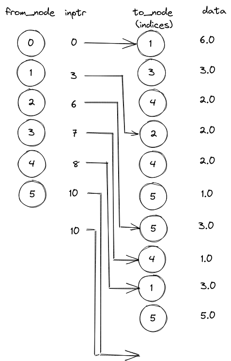
For a vertex tail_vert_idx, the head nodes of the outgoing edges are given by csr_indices[csr_indptr[tail_vert_idx]:csr_indptr[tail_vert_idx + 1]], and the associated attribute values by csr_data[csr_indptr[tail_vert_idx]:csr_indptr[tail_vert_idx + 1]]. For example:

tail_vert_idx = 0
print(
    f"head nodes: {csr_indices[csr_indptr[tail_vert_idx]:csr_indptr[tail_vert_idx + 1]]}"
)
print(
    f"edge weights: {csr_data[csr_indptr[tail_vert_idx]:csr_indptr[tail_vert_idx + 1]]}"
)

head nodes: [1 3 4]
edge weights: [6. 3. 2.]

It is also easy to loop over all the vertices and get the associated outgoing edges:

for tail_vert_idx in range(vertex_count):
    for indptr in range(csr_indptr[tail_vert_idx], csr_indptr[tail_vert_idx + 1]):
        head_vert_idx = csr_indices[indptr]
        edge_weight = csr_data[indptr]
        print(f"({tail_vert_idx},{head_vert_idx}) : {edge_weight}")

(0,1) : 6.0
(0,3) : 3.0
(0,4) : 2.0
(1,2) : 2.0
(1,4) : 2.0
(1,5) : 1.0
(2,5) : 3.0
(3,4) : 1.0
(4,1) : 3.0
(4,5) : 5.0

Next we are going to look at the Compressed Sparse Column (CSC) or Compressed Column Storage (CCS). This storage it directly related to the reverse star representation of a graph.

CSC format

Here is the description from netlib:

Analogous to Compressed Row Storage there is Compressed Column Storage (CCS), which is also called the Harwell-Boeing sparse matrix format. The CCS format is identical to the CRS format except that the columns of A are stored (traversed) instead of the rows. In other words, the CCS format is the CRS format for A.T.

The CCS format is specified by the 3 arrays {val, row_ind, col_ptr}, where row_ind stores the row indices of each nonzero, and col_ptr stores the index of the elements in val which start a column of A.

This time, the requirement is that the edge list in COO format must be sorted in an ascending way by the head node index.

edges_df.sort_values(by=["to_node", "from_node"], axis=0, ascending=True, inplace=True)
coo_row = edges_df["from_node"].values
coo_col = edges_df["to_node"].values
coo_val = edges_df["weight"].values

csc_indptr = np.zeros(vertex_count + 1, dtype=np.uint32)
csc_indices = np.zeros(edge_count, dtype=np.uint32)
csc_data = np.zeros(edge_count, dtype=np.float64)

for i in range(edge_count):
    csc_indptr[coo_col[i] + 1] += 1
    csc_indices[i] = coo_row[i]
    csc_data[i] = coo_val[i]

csc_indptr = np.cumsum(csc_indptr, dtype=np.uint32)

Check against SciPy:

sp_csc = sp_coo.tocsc()
assert np.allclose(csc_indptr, sp_csc.indptr)
assert np.allclose(csc_indices, sp_csc.indices)
assert np.allclose(csc_data, sp_csc.data)

csc_indptr

array([ 0,  0,  2,  3,  4,  7, 10], dtype=uint32)

csc_indices

array([0, 4, 1, 0, 0, 1, 3, 1, 2, 4], dtype=uint32)

csc_data

array([6., 3., 2., 3., 2., 2., 1., 1., 3., 5.])

With this CSC format, it is easy to get the incoming edges of a given vertex. For a vertex head_vert_idx, the tail nodes of the incoming edges are given by csc_indices[csc_indptr[head_vert_idx]:csc_indptr[head_vert_idx + 1]], and the associated attribute values by csc_data[csr_indptr[head_vert_idx]:csr_indptr[head_vert_idx + 1]]. For example:

head_vert_idx = 0
print(
    f"tail nodes: {csc_indices[csc_indptr[head_vert_idx]:csc_indptr[head_vert_idx + 1]]}"
)
print(
    f"edge weights: {csc_data[csc_indptr[head_vert_idx]:csc_indptr[head_vert_idx + 1]]}"
)

tail nodes: []
edge weights: []

This vertex has no incoming edge. We can try another one:

head_vert_idx = 4
print(
    f"tail nodes: {csc_indices[csc_indptr[head_vert_idx]:csc_indptr[head_vert_idx + 1]]}"
)
print(
    f"edge weights: {csc_data[csc_indptr[head_vert_idx]:csc_indptr[head_vert_idx + 1]]}"
)

tail nodes: [0 1 3]
edge weights: [2. 2. 1.]

Let’s loop over all the vertices and get the associated incoming edges:

for head_vert_idx in range(vertex_count):
    for indptr in range(csc_indptr[head_vert_idx], csc_indptr[head_vert_idx + 1]):
        tail_vert_idx = csc_indices[indptr]
        edge_weight = csc_data[indptr]
        print(f"({tail_vert_idx},{head_vert_idx}) : {edge_weight}")

(0,1) : 6.0
(4,1) : 3.0
(1,2) : 2.0
(0,3) : 3.0
(0,4) : 2.0
(1,4) : 2.0
(3,4) : 1.0
(1,5) : 1.0
(2,5) : 3.0
(4,5) : 5.0

Forward star and reverse star

So what do we call forward and reverse star exactly? Well this a generalization of the CSR and CSC format, with a pointer vector indptr of size (vertex_count + 1, 1) and an edge array of size (edge_count, n_att), where n_att is the number of edge attributes that we need to store. Note that we can store the head and tail indices in this array as edge attributes. In the case of forward star, indptr is pointing toward the outgoing edges, and in the case of the reverse star, toward the incoming edges. Here is a figure with a small example of a forward star (where the pointer vector is named point):

forward_star_example

Credit: these slides online. I guess that this comes from a book?

Because we are not dealing anymore with sparse matrices but directly with edges in triplet form, we can now handle parallel edges. Indeed, a 2D matrix can only have a single entry for a given row and column, but when the edge information is “unpivoted” in a triplet form, we can actually deal with duplicated entries with respect to head and tail nodes, and as many attributes as we want.

Let’s implement a function that converts an edge dataframe into a forward star object. The edge attributes are all assumed to be of float64 type. We would also like to store the head vertex indices in the edge array, but in NumPy, it is kind of complicated to handles 2D arrays with mixed column types (uint32 and float64). So here, we basically have an array of edge attributes with integer type (indices), and another one with the ones of float type. A C implementation could make use of some struct.

Edges dataframe to forward star

We assume that all the edge attributes are of float type.

def edges_to_FS(edges_df, from_node="from_node", to_node="to_node"):

    edges_df.sort_values(by=["from_node"], axis=0, ascending=True, inplace=True)

    vertex_count = edges_df[[from_node, to_node]].max().max() + 1
    edge_count = len(edges_df)

    attribute_count = edges_df.shape[1] - 2
    attribute_names = [c for c in edges_df.columns if c not in [from_node, to_node]]

    from_node = edges_df[from_node].values
    to_node = edges_df[to_node].values
    edge_val = edges_df[attribute_names].values

    csr_indptr = np.zeros(vertex_count + 1, dtype=np.uint32)
    csr_indices = np.zeros(edge_count, dtype=np.uint32)
    csr_data = np.zeros((edge_count, attribute_count), dtype=np.float64)
    for i in range(edge_count):
        csr_indptr[from_node[i] + 1] += 1
        csr_indices[i] = to_node[i]
        csr_data[i] = edge_val[i]
    csr_indptr = np.cumsum(csr_indptr, dtype=np.uint32)

    names = ",".join(attribute_names)
    csr_data = np.core.records.fromarrays(csr_data.T, names=names)

    FS = namedtuple("FS", ["indptr", "indices", "data"])
    return FS(csr_indptr, csr_indices, csr_data)

FS = edges_to_FS(edges_df)

FS.indptr

array([ 0,  3,  6,  7,  8, 10, 10], dtype=uint32)

FS.indices

array([1, 3, 4, 2, 4, 5, 5, 4, 1, 5], dtype=uint32)

FS.data

rec.array([(6.,), (3.,), (2.,), (2.,), (2.,), (1.,), (3.,), (1.,), (3.,),
           (5.,)],
          dtype=[('weight', '<f8')])

Let’s finish with a small example, with some kind of special features.

Example with parallel edges, a loop, an isolated vertex and several edge attributes

query_1

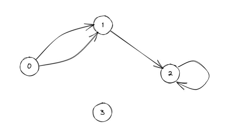
tail_verts = np.array([0, 0, 1, 3], dtype=np.uint32)
head_verts = np.array([1, 1, 3, 3], dtype=np.uint32)
edge_a1 = np.array([2, 1, 2, 3], dtype=np.float64)
edge_a2 = np.array([3, 2, 8, 9], dtype=np.float64)
edge_a3 = np.array([0.1, 0.6, 0.4, 0.0], dtype=np.float64)
edges_df = pd.DataFrame(
    data={
        "from_node": tail_verts,
        "to_node": head_verts,
        "a_1": edge_a1,
        "a_2": edge_a2,
        "a_3": edge_a3,
    }
)

edges_df.head(4)

	from_node	to_node	a_1	a_2	a_3
0	0	1	2.0	3.0	0.1
1	0	1	1.0	2.0	0.6
2	1	3	2.0	8.0	0.4
3	3	3	3.0	9.0	0.0

vertex_count = edges_df[["from_node", "to_node"]].max().max() + 1
edge_count = len(edges_df)
print(f"vertex count : {vertex_count},  edge count : {edge_count}")

vertex count : 4,  edge count : 4

fs = edges_to_FS(edges_df)

for tail_vert_idx in range(vertex_count):
    for indptr in range(fs.indptr[tail_vert_idx], fs.indptr[tail_vert_idx + 1]):
        head_vert_idx = fs.indices[indptr]
        edge_data = fs.data[indptr]
        print(f"({tail_vert_idx},{head_vert_idx}) : {edge_data}")

(0,1) : (2., 3., 0.1)
(0,1) : (1., 2., 0.6)
(1,3) : (2., 8., 0.4)
(3,3) : (3., 9., 0.)

Everything seems to be OK.

In another post, we will see how to implement the forward and reverse stars efficiently in Cython and compare this data structure with another one.

References

[1] Y. Sheffi, “Urban Transportation Networks: Equilibrium Analysis with Mathematical Programming Methods,” Prentice-Hall, Englewoods Cliffs, 1985.