Visualizing some polynomial roots with Datashader

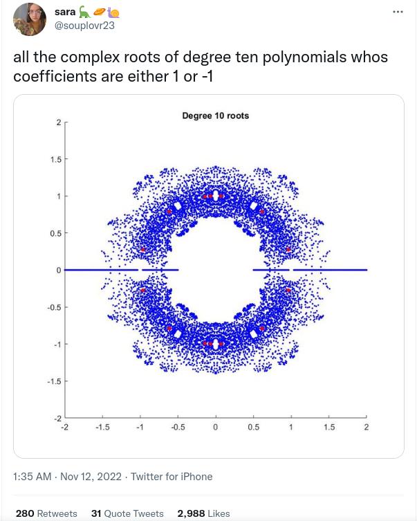
Last week-end I found this interesting tweet by sara:

The above figure shows all the complex roots from the various polynomials of degree 10 with coefficients in the set $\left\{ -1, 1 \right\}$. It made me think of Bohemian matrix eigenvalues, and I guess it is related (through the polynomial’s companion matrix).

If we think of the general polynomial:

\[P(x) = \sum_{i=0}^m a_i \; x^{m-i}\]

we have in the above tweet, $m=10$ and $a_i \in \left\{-1 , 1 \right\}, \; \forall i \geq 0$. We are going to keep this set of possible values for the polynomial coefficients, but increase the polynomial degree $m$ a little bit.

The roots of $P(x)$ are going to be computed with NumPy and Cython (we could have done it with Numba as well). Then we are going to visualize the point density in the complex plane with datashader, which is the appropriate tool in Python for such a visualization I think.

Imports

import colorcet
import datashader as ds
import numpy as np
import pandas as pd
from datashader import tf

%load_ext cython

Package versions:

Python version       : 3.10.6
colorcet             : 3.0.1
cython               : 0.29.32
datashader           : 0.14.2
numpy                : 1.23.4
pandas               : 1.5.1
OS                   : Linux

Cartesian product of all coefficient values

We first evaluate the number of distinct polynomials with coefficients in the given set. This corresponds to a Cartesian product of the provided set $\left\{-1 , 1 \right\}$ with itself $m+1$ times:

coef_values = [-1, +1]
coef_values_np = np.array(coef_values, dtype=np.int8)

m = 23  # degree of the polynomial
n = np.power(len(coef_values), m + 1)
print(f"we have {n} distinct polynomials of degree {m}")

we have 16777216 distinct polynomials of degree 23

With np.roots, the polynomials $P(x) = a_0 \; x^m + a_1 \; x^{m-1} + … + a_{m-1} \; x + a_m$ are only defined by the coefficients, in this order:

\[\left[a_0 \; a_1 \; ... \; a_{m-1} \; a_m\right]\]

Let’s generate the coefficient values:

poly_coefs_all = np.stack(np.meshgrid(*((m+1) * [coef_values_np])), -1).reshape(-1, m+1)

for poly_coefs in poly_coefs_all[:5]:
    print(poly_coefs)

[-1 -1 -1 -1 -1 -1 -1 -1 -1 -1 -1 -1 -1 -1 -1 -1 -1 -1 -1 -1 -1 -1 -1 -1]
[-1 -1 -1 -1 -1 -1 -1 -1 -1 -1 -1 -1 -1 -1 -1 -1 -1 -1 -1 -1 -1 -1 -1  1]
[-1 -1 -1 -1 -1 -1 -1 -1 -1 -1 -1 -1 -1 -1 -1 -1 -1 -1 -1 -1 -1 -1  1 -1]
[-1 -1 -1 -1 -1 -1 -1 -1 -1 -1 -1 -1 -1 -1 -1 -1 -1 -1 -1 -1 -1 -1  1  1]
[-1 -1 -1 -1 -1 -1 -1 -1 -1 -1 -1 -1 -1 -1 -1 -1 -1 -1 -1 -1 -1  1 -1 -1]

poly_coefs_all.shape

(16777216, 24)

Polynomial roots

Now we compute the roots of each of the 16777216 polynomials:

%%cython --compile-args=-Ofast
# cython: language_level=3, boundscheck=False, wraparound=False, embedsignature=False, initializedcheck=False

import numpy as np

cimport numpy as cnp


cdef void loop_over_polys_cython(cnp.complex128_t[:,:] roots_all, cnp.int8_t[:,:] poly_coefs_all, ssize_t n, ssize_t m):
    
    cdef: 
        ssize_t i, j

    roots = np.empty(m-1, dtype=np.complex128)
    for i in range(n):
        roots = np.roots(np.array(poly_coefs_all[i, :], dtype=np.float64))
        for j in range(m-1):
            roots_all[i, j] = <cnp.complex64_t>roots[j]

cpdef loop_over_polys(poly_coefs_all):
    cdef:
        ssize_t n = <ssize_t>poly_coefs_all.shape[0]
        ssize_t m = <ssize_t>poly_coefs_all.shape[1]
        
    roots_all = np.empty((n, m-1), dtype=np.complex128)
    
    cdef cnp.complex128_t[:,:] roots_all_view = roots_all
    loop_over_polys_cython(roots_all_view, poly_coefs_all, n, m)
    return roots_all

This computation could be done in parallel: we could assign some chunks of polynomials to each job. However, this is sequential in the present short post. Since the roots are computed with NumPy on the Python level, we cannot release the GIL and use a prange loop from Cython. The computation takes around 43 minutes on my laptop.

%%time
roots_all = loop_over_polys(poly_coefs_all)

CPU times: user 43min 50s, sys: 6.1 s, total: 43min 56s
Wall time: 43min 48s

roots_all.shape

(16777216, 23)

We transform the 2D array into a 1D array:

roots_all = roots_all.flatten()

roots_all.shape

(385875968,)

roots_all[:5]

array([0.96592581+0.25881904j, 0.96592581-0.25881904j,
       0.86602539+0.5j       , 0.86602539-0.5j       ,
       0.70710677+0.70710677j])

Plot with datashader

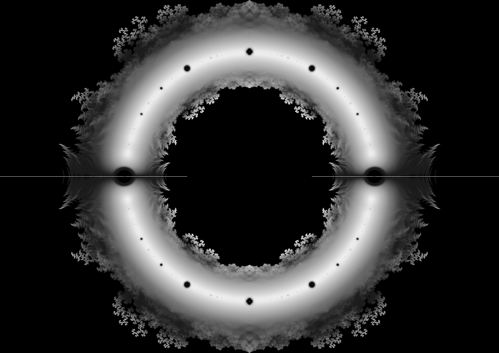
Finally, we separate the real and imaginary part of the roots, load them into a Pandas dataframe and plot them with datashader.

df = pd.DataFrame(data={"x": roots_all.real, "y": roots_all.imag})

plot_width = 1600
plot_height = int(
    np.round((df.y.max() - df.y.min()) * plot_width / (df.x.max() - df.x.min()))
)
cvs = ds.Canvas(plot_width=plot_width, plot_height=plot_height)
agg = cvs.points(df, "x", "y")
img = ds.tf.shade(agg, cmap=colorcet.dimgray, how="eq_hist")
img = tf.set_background(img, "black")
img

datashader