Using a local sentence embedding model for similarity calculation
A simple yet powerful use case of sentence embeddings is computing the similarity between different sentences. By representing sentences as numerical vectors, we can leverage mathematical operations to determine the degree of similarity.
For the purpose of this demonstration, we’ll be using a recent text embedding model provided by the Beijing Academy of Artificial Intelligence (BAAI): BAAI/bge-base-en. BGE stands for BAAI General Embedding, and appears to be a BERT-like family of models, with a MIT licence. This particular model exhibits an embedding dimension of 768 and an input sequence length of 512 tokens. Keep in mind that longer sequences are truncated to fit within this limit. To put things into perspective, let’s compare it to OpenAI’s well-known model: text-embedding-ada-002, which features an embedding dimension of 1536 and an input sequence length of 8191 tokens. While the latter model offers some impressive capabilities, it’s worth noting that it cannot be run locally. Here’s a quick comparison of these two embedding models:
| Model | Can Run Locally | Multilingual | Input Sequence Length | Embedding Dimension |
|---|---|---|---|---|
BAAI/bge-base-en |
Yes | No | 512 | 768 |
text-embedding-ada-002 |
No | Yes | 8191 | 1536 |
While a larger instance of BAAI/bge - BAAI/bge-large-en - is available, we’ve opted for BAAI/bge-base-en for its relatively smaller size of 0.44GB, making it fast and suitable for regular machines. It’s also worth mentioning that despite its compact nature, BAAI/bge-base-en boasts a second-place rank on the Massive Text Embedding Benchmark leaderboard MTEB at the time of writing this post, which you can check out here: https://huggingface.co/spaces/mteb/leaderboard.
For the purpose of running this embedding model, we’ll be utilizing the neat Python library sentence_transformers. Alternatively, there are other Python libraries that provide access to this model, such as FlagEmbedding or LangChain.
Now, let’s get started by importing the necessary libraries.
Imports
import matplotlib.pyplot as plt
import numpy as np
import pandas as pd
import seaborn as sns
from sentence_transformers import SentenceTransformer
System information and package versions:
Python version       : 3.11.4
OS                   : Linux
Machine              : x86_64
matplotlib           : 3.7.1
numpy                : 1.24.4
pandas               : 2.0.3
seaborn              : 0.12.2
sentence_transformers: 2.2.2
Download and load the embedding model
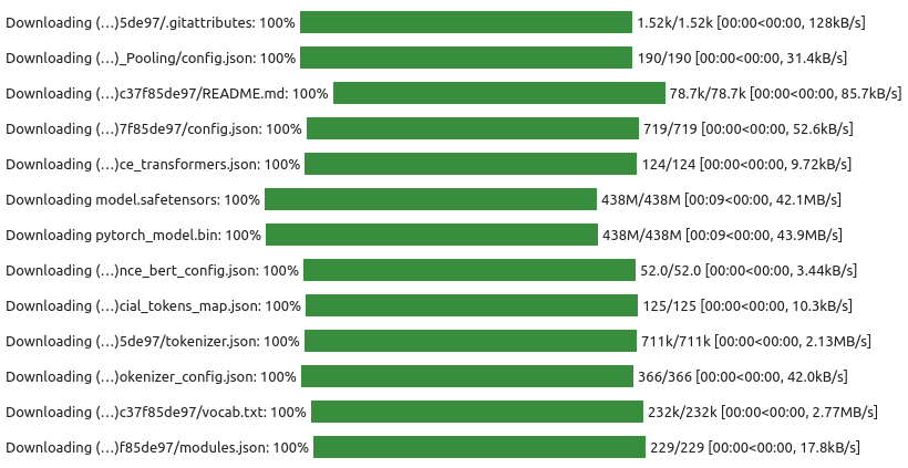
To get started with sentence embeddings, we’ll need to download and load the BAAI/bge-base-en model using the SentenceTransformer library. If it’s the first time you’re using this model, executing the following code will trigger the download of various files:
model = SentenceTransformer('BAAI/bge-base-en')

The model’s artifacts are cached in a hidden home directory:
$ tree ~/.cache/torch/sentence_transformers/BAAI_bge-base-en
.cache/torch/sentence_transformers/BAAI_bge-base-en
├── 1_Pooling
│   └── config.json
├── config.json
├── config_sentence_transformers.json
├── model.safetensors
├── modules.json
├── pytorch_model.bin
├── README.md
├── sentence_bert_config.json
├── special_tokens_map.json
├── tokenizer_config.json
├── tokenizer.json
└── vocab.txt

1 directory, 12 files
With the model loaded, we’re now ready to encode our first sentence. The resulting embedding vector is an array of floating-point values:
emb = model.encode("It’s not an easy thing to meet your maker", normalize_embeddings=True)
emb[:5]
array([-0.01139987,  0.00527102, -0.00226131, -0.01054202,  0.04873622],
      dtype=float32)
We can check the dimensions of the embedding and confirm that the vector has been normalized:
emb.shape
(768,)
np.linalg.norm(emb, ord=2)
0.99999994
Next we’ll compute embeddings for two sentences and then measure their cosine similarity.
Cosine similarity
In order to compute an embedding, we’ll use a helper function that can be expanded upon in the future to clean the input text. For now, it only removes any carriage returns and line feeds from the input text:
def get_embedding(text, normalize=True):
    text = text.replace("\r", " ").replace("\n", " ")
    return model.encode(text, normalize_embeddings=normalize)
Let’s start by creating an empty list to store the resulting embeddings:
embs = []
Now we compute two embeddings:
# first sentence
sen_1 = "Berlin is the capital of Germany"
emb_1 = get_embedding(sen_1)
embs.append((sen_1, emb_1))

# second sentence
sen_2 = "Yaoundé is the capital of Cameroon"
emb_2 = get_embedding(sen_2)
embs.append((sen_2, emb_2))
With the embeddings computed, we can now move on to calculating their cosine similarity. The cosine similarity $S(u,v)$ between two vectors $u$ and $v$ is defined as:
\[S(u, v) = cos(u, v) = \frac{u \cdot v}{\|u\|_2 \|v\|_2}\]def cosine_similarity(vec1, vec2, normalized=True):
if normalized:
return np.dot(vec1, vec2)
else:
return np.dot(vec1, vec2) / (
np.linalg.norm(vec1, ord=2) * np.linalg.norm(vec2, ord=2)
)
Cosine similarity values range between -1 and 1. When applied to the same vector, the result is 1:
cosine_similarity(emb_1, emb_1)
1.0000001
When applied to opposite vectors, the result is -1:
cosine_similarity(-emb_1, emb_1)
-1.0000001
If the result is close to zero, it indicates that the vectors are nearly orthogonal:
cosine_similarity(emb_1, emb_2 - np.dot(emb_1, emb_2) * emb_1)
-4.4703484e-08
Remember that the concept of cosine similarity is tied to angles. Even when vectors have different magnitudes, collinear vectors are perceived as similar. It’s important to note that $S(u,v) = 1$ indicates that $u = v$, only when working with vectors of same magnitude. Another related measure is cosine distance: $d(u,v) = 1 - S(u,v)$. However, it’s worth mentioning that cosine distance doesn’t qualify as a metric due to its failure to meet the triangle inequality requirement: $d(u, v) \leq d(u, w) + d(w, v)$ for any $w$.
And here is the cosine similarity between the embeddings of the two sentences computed above:
cosine_similarity(emb_1, emb_2)
0.8196905
This seems to be a rather large similarity value.
Cosine similarity heatmaps
Let’s take this a step further by generating a cosine similarity heatmap. To begin, we’ll compute embeddings for three additional sentences:
sen_3 = "Esplanade MRT station is an underground Mass Rapid Transit station on the Circle line in Singapore"
emb_3 = get_embedding(sen_3)
embs.append((sen_3, emb_3))
sen_4 = "Remove jalapeños from surface and stir in the additional chili powder, ground cumin and onion powder."
emb_4 = get_embedding(sen_4)
embs.append((sen_4, emb_4))
sen_5 = "Fideua is a traditional dish, similar in style to paella but made with short spaghetti-like pasta."
emb_5 = get_embedding(sen_5)
embs.append((sen_5, emb_5))
With the embeddings computed, we can now proceed to calculate a 5-by-5 similarity matrix that compares the embeddings of all the stored sentences. Here’s how we can do it:
def compute_cosine_similarity_matrix(embs, label_size=30):
    l = len(embs)
    cds = np.zeros((l, l), dtype=np.float64)
    for i, (_, emb) in enumerate(embs):
        cds[i, i] = 0.5
        for j in range(i + 1, l):
            cs = cosine_similarity(emb, embs[j][1], normalized=True)
            cds[i, j] = cs
    # The matrix is symmetric with unit diagonal
    cds += np.transpose(cds)
    labels = [t[0][:label_size] + "..." for t in embs]
    df = pd.DataFrame(data=cds, index=labels, columns=labels)
    return df


df = compute_cosine_similarity_matrix(embs)
df
| Berlin is the capital of Germa... | Yaoundé is the capital of Came... | Esplanade MRT station is an un... | Remove jalapeños from surface ... | Fideua is a traditional dish, ... | |
|---|---|---|---|---|---|
| Berlin is the capital of Germa... | 1.000000 | 0.819691 | 0.711520 | 0.685216 | 0.701959 |
| Yaoundé is the capital of Came... | 0.819691 | 1.000000 | 0.702962 | 0.673310 | 0.714926 |
| Esplanade MRT station is an un... | 0.711520 | 0.702962 | 1.000000 | 0.655668 | 0.625339 |
| Remove jalapeños from surface ... | 0.685216 | 0.673310 | 0.655668 | 1.000000 | 0.757284 |
| Fideua is a traditional dish, ... | 0.701959 | 0.714926 | 0.625339 | 0.757284 | 1.000000 |
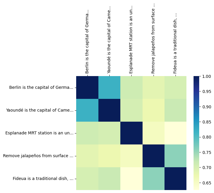
To visualize this information, we create a heatmap using Seaborn:
fig, ax = plt.subplots(figsize=(6, 5))
ax = sns.heatmap(df, cmap="YlGnBu")
ax.xaxis.tick_top()
for label in ax.get_xticklabels():
    label.set_rotation(90)

Darker shades indicate higher cosine similarity values, highlighting sentences that are more semantically similar to each other. Sentences related to country capitals or food exhibit a larger cross similarity than others.
Let’s further illustrate the concept of cosine similarity by applying it to a different set of sentences centered around the message: “I love pizza”. We’ll start by creating embeddings for the following set of sentences:
sentences = [
    "I love pizza",
    "i love Pizza",
    "i have a passion for Pizza",
    "I like pizza",
    "Pizza is my favorite food",
    "I think pizza is yummy!",
    "I love eating pizza",
    "I love to eat pizza",
    "I like eating pizza",
    "I am obsessed with pizza",
    "I am addicted to pizza",
    "Uranium-235 has a half-life of 703.8 million years",
    "I HATE pizza",
    "Pizza is disgusting!",
    "Pizza is a horrible food",
]
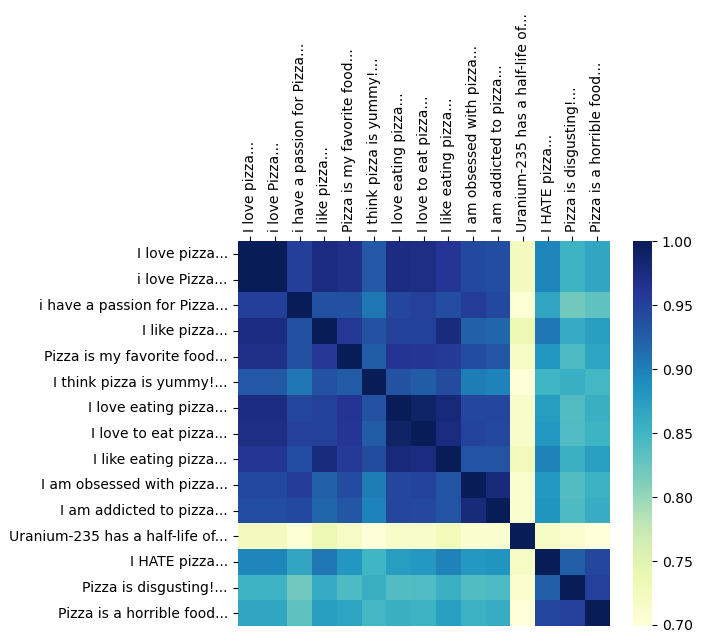
After encoding these sentences, we’ll compute the cosine similarity matrix and visualize it with a heatmap:
embeddings = model.encode(sentences, normalize_embeddings=True)
df = compute_cosine_similarity_matrix(list(zip(sentences, embeddings)))
fig, ax = plt.subplots(figsize=(6, 5))
ax = sns.heatmap(df, cmap="YlGnBu")
ax.xaxis.tick_top()
for label in ax.get_xticklabels():
    label.set_rotation(90)

Sentences expressing positive sentiments about pizza cluster together, forming regions of higher cosine similarity, while negative sentiments are distinctly separated. It’s worth mentioning that one of the applications of sentence embedding models is sentiment analysis. We can also observe that the “Uranium-235” sentence is not related to the other sentences.
Encoding processing time
Performance is a crucial consideration when working with real-world datasets. Let’s take a moment to evaluate the encoding processing time of the sentence embedding model on a regular GPU. For this purpose, we’ll encode a list of 100,000 identical sentences. While this might seem repetitive, and the chosen sentence is kind of short, this will provide us with a very rough estimate of the time it takes to encode a larger list of sentences.
sentences = 100_000 * ["All work and no play makes Jack a dull boy"]
%%time
embeddings = model.encode(sentences, normalize_embeddings=True)
CPU times: user 46.7 s, sys: 3.48 s, total: 50.2 s
Wall time: 37 s
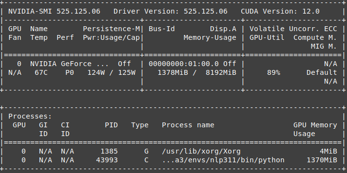
The GPU is a NVIDIA GeForce RTX 3070 Ti Laptop with 8GB of memory:

So it takes 37s to encode these 100,000 short sentences.
Conclusion
In this very short exploration of sentence embeddings, we’ve delved into the world of transforming textual information into meaningful numerical representations. One standout feature that makes this technology truly accessible is the ability to run open-source models locally, putting the power of sentence embeddings right at your fingertips.