Calculating daily mean temperatures with scikit-learn
The goal is of this post is to predict the daily mean air temperature TAVG from the following climate data variables: maximum and minimum daily temperatures and daily precipitation, using Python and some machine learning techniques available in scikit-learn.
Our dataset comes from the Climate Data Online Search provided by the National Centers for Environmental Information (NCEI), a U.S. government agency that manages an extensive archive of atmospheric, coastal, geophysical, and oceanic data. Specifically, they have gathered data from the Lyon station, located at the Saint-Exupéry airport, spanning from 1920 to the present day.
The key variables we’ll be working with are:
PRCP = Precipitation (tenths of mm)
TMAX = Maximum temperature (tenths of degrees C)
TMIN = Minimum temperature (tenths of degrees C)
TAVG = Average temperature (tenths of degrees C)
  [Note that TAVG from source 'S' corresponds
   to an average for the period ending at
   2400 UTC rather than local midnight]
The description above can be found in the dataset documentation.
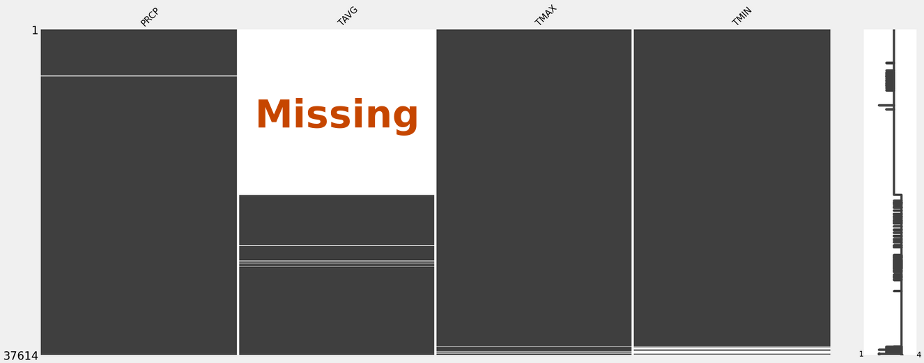
However, a significant portion of the TAVG data is missing. The dataset has 37614 rows and 5 columns: DATE, PRCP, TAVG, TMAX and TMIN, and TAVG is missing for more that half of the time range:
Our initial strategy involves calculating TAVG as the arithmetic mean of TMAX and TMIN, but this is not the best option. Here is a excerpt from the dissertation abstract by Jase Bernhardt [1] about this traditional approach:
Traditionally, daily average temperature is computed by taking the mean of two values- the maximum temperature over a 24-hour period and the minimum temperature over the same period. These data form the basis for numerous studies of long-term climatologies (e.g. 30-year normals) and recent temperature trends and changes. However, many first-order weather stations (e.g. airports) also record hourly temperature data. Using an average of the 24 hourly temperature readings to compute daily average temperature should provide a more precise and representative estimate of a given day’s temperature. These two methods of daily temperature averaging ([Tmax + Tmin]/2, average of 24 hourly temperature values) were computed and mapped for all first-order weather stations across the United States for the 30-year period 1981-2010. This analysis indicates a statistically significant difference between the two methods, as well as an overestimation of temperature by the traditional method ([Tmax + Tmin]/2), particularly in southern and coastal portions of the Continental U.S. The likely explanation for the long-term difference between the two methods is the underlying assumption of the twice-daily method that the diurnal curve of temperature follows a symmetrical pattern.
In this post, we’ll go through feature engineering: extract temporal features, compute the diurnal temperature range (DTR), consider daylight duration, and calculate the deltas of TMIN and TMAX with the previous and next days. We’ll evaluate the performance of different models, including:
- Baseline Model: Arithmetic mean of TMIN and TMAX
- Ridge Regression
- Decision Tree Regressor
- Random Forest Regressor
- Histogram-based Gradient Boosting Regressor
We’ll assess these models using mean absolute error (MAE) and root mean squared error (RMSE) to determine which one provides the most accurate predictions for TAVG, with the baseline being the arithmetic mean of TMIN and TMAX.
Imports
Let’s start by gathering the tools we need in the following:
import warnings

import matplotlib.pyplot as plt
import missingno as msno
import numpy as np
import pandas as pd
from astral import Observer
from astral.sun import daylight
from optuna import create_study
from optuna.exceptions import ExperimentalWarning
from optuna.samplers import NSGAIISampler
from sklearn.ensemble import HistGradientBoostingRegressor, RandomForestRegressor
from sklearn.linear_model import LinearRegression, Ridge
from sklearn.metrics import mean_absolute_error, mean_squared_error
from sklearn.model_selection import KFold, cross_val_score, train_test_split
from sklearn.pipeline import Pipeline
from sklearn.preprocessing import StandardScaler
from sklearn.tree import DecisionTreeRegressor
from sklego.preprocessing import RepeatingBasisFunction

warnings.filterwarnings("ignore", category=ExperimentalWarning)
plt.style.use("fivethirtyeight")

temperature_fp = "./3441363.csv"
RS = 124  # random seed
FS = (9, 6)  # figure size
OS and package versions:
Python version       : 3.11.5
OS                   : Linux
Machine              : x86_64
matplotlib           : 3.7.2
numpy                : 1.24.4
pandas               : 2.1.0
astral               : 3.2
optuna               : 3.3.0
sklearn              : 1.3.0
Load the data
Let’s start by loading the data we’ll be working with, downloaded as a CSV file:
df = pd.read_csv(temperature_fp)  # Load the dataset and select the relevant columns
station = df[["STATION", "NAME", "LATITUDE", "LONGITUDE", "ELEVATION"]].iloc[0]
df = df[["DATE", "PRCP", "TAVG", "TMIN", "TMAX"]].dropna(how="all")

# Convert the 'DATE' column to a datetime format and set it as the index
df.DATE = pd.to_datetime(df.DATE)
df.set_index("DATE", inplace=True)
df = df.asfreq("D")
df.sort_index(inplace=True)

df.head(3)
| PRCP | TAVG | TMIN | TMAX | |
|---|---|---|---|---|
| DATE | ||||
| 1920-09-01 | 0.0 | NaN | 8.8 | 19.7 |
| 1920-09-02 | 0.0 | NaN | 9.1 | 20.1 |
| 1920-09-03 | 1.5 | NaN | 9.3 | 16.8 |
Now, let’s take a closer look at the dataset’s dimensions:
df.shape
(37617, 4)
This corresponds to approximately 103 years of daily data. We also got some information about the weather station:
station
STATION              FR069029001
NAME         LYON ST EXUPERY, FR
LATITUDE                 45.7264
LONGITUDE                 5.0778
ELEVATION                  235.0
Name: 0, dtype: object
It’s worth noting a peculiar aspect of the data: the daily mean temperature can sometimes be slightly smaller than the daily minimum temperature:
len(df[df.TAVG < df.TMIN])
31
And, on occasion, it can surpass the daily maximum temperature:
len(df[df.TAVG > df.TMAX])
235
This intriguing phenomenon may be attributed to measurement methods and the consideration that TAVG corresponds to an average for the period ending at 2400 UTC rather than local midnight.
Now let’s take a closer look at missing values within our dataset:
ax = (100 * df.isna().sum(axis=0) / len(df)).plot.bar(alpha=0.7, figsize=(6, 3))
_ = ax.set_ylim(0, 60)
_ = ax.set(
    title="Ratio of missing values per column", xlabel="Column name", ylabel="Ratio (%)"
)
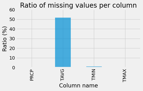
We will utilize segments of the existing TAVG data as both training and testing datasets, with the ultimate aim of predicting the absent values.
First approach : TAVG_am, arithmetic mean of TMIN and TMAX
Let’s kick off our analysis by introducing TAVG_am, which represents the arithmetic mean of TMIN and TMAX:
df["TAVG_am"] = 0.5 * (df["TMIN"] + df["TMAX"])
ax = df[["TAVG", "TAVG_am"]].plot.scatter(
    x="TAVG", y="TAVG_am", alpha=0.2, figsize=(6, 6)
)

df_tmp = df[["TAVG", "TAVG_am"]].dropna(how="any")
X = df_tmp["TAVG"].values[:, np.newaxis]
y = df_tmp["TAVG_am"].values
lr = LinearRegression()
lr.fit(X, y)

x_min, x_max = -11, 36
points = np.linspace(x_min, x_max, 100)
_ = ax.plot(points, points, color="r")
_ = plt.plot(X, lr.predict(X), color="k", linewidth=1)
_ = ax.set_xlim(x_min, x_max)
_ = ax.set_ylim(x_min, x_max)
_ = ax.legend(["TAVG, TAVG_am couples", "y=x", "Linear regression"])
_ = ax.set(title="Correlation between TAVG and TAVG_am")
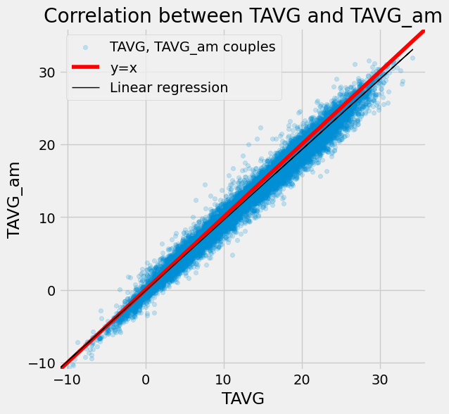
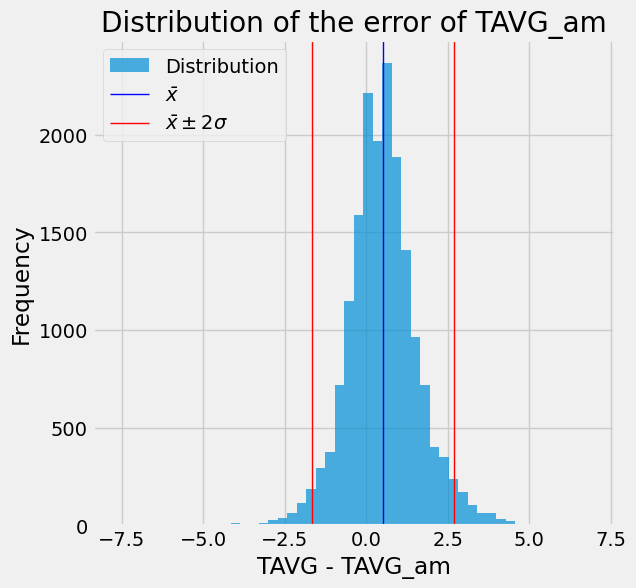
As seen in the scatter plot above, there’s a clear correlation between TAVG and TAVG_am. However, we can observe that TAVG_am may underestimate TAVG by around 3 or 4 degrees. To delve deeper into this discrepancy, let’s examine the error distribution between TAVG and TAVG_am:
diff = (df.TAVG - df.TAVG_am).dropna()
avg = diff.mean()
std = diff.std()
ax = diff.plot.hist(bins=50, alpha=0.7, figsize=(6, 6))
_ = plt.axvline(x=avg, color="b", linewidth=1)
_ = plt.axvline(x=avg - 2 * std, color="r", linewidth=1)
_ = plt.axvline(x=avg + 2 * std, color="r", linewidth=1)
ax.legend(["Distribution", "$\\bar{x}$", "$\\bar{x} \pm 2 \sigma$"])
_ = ax.set(title="Distribution of the error of TAVG_am", xlabel="TAVG - TAVG_am")
Model evaluation
In order to assess the performance of our model, we’ve defined a convenient evaluation function:
def evaluate(y_true, y_pred, return_score=False):
    d = {}
    d["mae"] = mean_absolute_error(y_true, y_pred)
    d["rmse"] = mean_squared_error(y_true, y_pred, squared=False)
    if return_score:
        return d
    else:
        print(
            f'Mean absolute error : {d["mae"]:8.4f}, Mean squared error : {d["rmse"]:8.4f}'
        )
This function computes two important metrics:
- Mean Absolute Error (MAE)
- Root Mean Squared Error (RMSE)
Now, let’s apply this evaluation function to our model predictions:
y_pred = df.loc[~df.TAVG.isna() & ~df.TAVG_am.isna(), "TAVG_am"].values
y_true = df.loc[~df.TAVG.isna() & ~df.TAVG_am.isna(), "TAVG"].values
evaluate(y_true, y_pred)
Mean absolute error : 0.9098, Mean squared error : 1.2088
This gives us an idea of the baseline score, which we are going to improve.
# cleanup: remove the temporary TAVG_am column
df.drop("TAVG_am", axis=1, inplace=True)
Feature engineering
Let’s add the following features to the dataset:
- Cyclic time data encoding
- Diurnal Temperature Range (DTR)
- Daylight length
- TMIN and TMAX delta with adjacent days
Temporal features
df.reset_index(drop=False, inplace=True)
df["year"] = df["DATE"].dt.year
df["month"] = df["DATE"].dt.month
df["dayofyear"] = df["DATE"].dt.dayofyear
df.set_index("DATE", inplace=True)
df.head(3)
| PRCP | TAVG | TMIN | TMAX | year | month | dayofyear | |
|---|---|---|---|---|---|---|---|
| DATE | |||||||
| 1920-09-01 | 0.0 | NaN | 8.8 | 19.7 | 1920 | 9 | 245 |
| 1920-09-02 | 0.0 | NaN | 9.1 | 20.1 | 1920 | 9 | 246 |
| 1920-09-03 | 1.5 | NaN | 9.3 | 16.8 | 1920 | 9 | 247 |
df["daycountinyear"] = df["year"].map(lambda y: pd.Timestamp(y, 12, 31).dayofyear)
df["sin_encoded_year"] = np.sin(
    2.0 * np.pi * (df["dayofyear"] - 1) / df["daycountinyear"]
)
df["cos_encoded_year"] = np.cos(
    2.0 * np.pi * (df["dayofyear"] - 1) / df["daycountinyear"]
)
df.drop(["year", "daycountinyear"], axis=1, inplace=True)
ax = df["2020":"2020"][["sin_encoded_year", "cos_encoded_year"]].plot(figsize=(6, 3))
_ = ax.set(title="Cyclical encoded day-of-year", xlabel="Day-of-year")

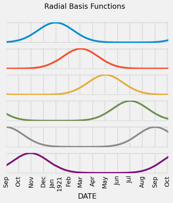
Radial basis functions:
rbf = RepeatingBasisFunction(
    n_periods=6, column="dayofyear", input_range=(1, 366), remainder="drop"
)
rbf.fit(df)
RBFs = pd.DataFrame(index=df.index, data=rbf.transform(df))
RBFs = RBFs.add_prefix("rbf_")
axs = RBFs[:400].plot(
    subplots=True,
    figsize=(6, 6),
    sharex=True,
    title="Radial Basis Functions",
    legend=False,
    rot=90,
)
for ax in axs:
    ax.yaxis.set_tick_params(labelleft=False)
df = pd.concat((df, RBFs), axis=1)
Temperature ranges, deltas with previous and next days
Daily temperature range:
df["DTR"] = df["TMAX"] - df["TMIN"]
TMIN and TMAX deltas with previous and next days:
df["TMAX_day_before"] = df["TMAX"].shift(+1)
df["TMIN_day_before"] = df["TMIN"].shift(+1)
df["TMAX_day_after"] = df["TMAX"].shift(-1)
df["TMIN_day_after"] = df["TMIN"].shift(-1)
df["TMAX_delta_db"] = df["TMAX"] - df["TMAX_day_before"]
df["TMIN_delta_db"] = df["TMIN"] - df["TMIN_day_before"]
df["TMAX_delta_da"] = df["TMAX"] - df["TMAX_day_after"]
df["TMIN_delta_da"] = df["TMIN"] - df["TMIN_day_after"]
df.drop(
    ["TMIN_day_before", "TMAX_day_before", "TMIN_day_after", "TMAX_day_after"],
    axis=1,
    inplace=True,
)
Daytime length
observer = Observer(latitude=station.LATITUDE, longitude=station.LONGITUDE)


def compute_daytime(date):
    sr, ss = daylight(observer, date=date)
    return (ss - sr).total_seconds()


df["datetime"] = df.index
df["daytime"] = df["datetime"].map(lambda d: compute_daytime(d))
df.drop("datetime", axis=1, inplace=True)
Train/test split
In this section, we split our dataset into two distinct sets – the training set and the testing set. First, we identify our target variable, which is what we want to predict – TAVG. We also define our features, which are the input variables used to make predictions.
target = "TAVG"
features = [c for c in df.columns if c != target]
features
['PRCP',
 'TMIN',
 'TMAX',
 'month',
 'dayofyear',
 'sin_encoded_year',
 'cos_encoded_year',
 'rbf_0',
 'rbf_1',
 'rbf_2',
 'rbf_3',
 'rbf_4',
 'rbf_5',
 'DTR',
 'TMAX_delta_db',
 'TMIN_delta_db',
 'TMAX_delta_da',
 'TMIN_delta_da',
 'daytime']
dataset = df[~df.TAVG.isna()].copy(deep=True)
dataset.dropna(how="any", inplace=True)
X, y = dataset[features].copy(deep=True), dataset[target].copy(deep=True)
X_train, X_test, y_train, y_test = train_test_split(
    X, y, test_size=0.3, random_state=RS, shuffle=True
)
Baseline : arithmetic mean
In this section, we establish a simple baseline model for predicting the average temperature with the arithmetic mean:
class BaselineModel:
    def fit(self, X_train):
        pass

    def predict(self, X_test):
        if "TAVG_am" in X_test:
            return X_test["TAVG_am"].values
        else:
            return 0.5 * (X_test["TMIN"].values + X_test["TMAX"].values)
baseline = BaselineModel()
y_pred = baseline.predict(X_test)
results = pd.DataFrame()
results = pd.concat(
    [
        results,
        pd.Series(evaluate(y_test, y_pred, return_score=True)).to_frame("baseline").T,
    ],
    axis=0,
)
results
| mae | rmse | |
|---|---|---|
| baseline | 0.916753 | 1.214852 |
Ridge
Now we introduce our first predictive model: Ridge Regression. Ridge Regression is a linear regression variant that is particularly useful when dealing with multicollinearity in the data.
ridge_reg = Pipeline(
    [
        ("scaler", StandardScaler()),
        ("ridge", Ridge(alpha=1.0)),
    ]
)
ridge_reg.fit(X_train, y_train)
y_pred = ridge_reg.predict(X_test)
results = pd.concat(
    [
        results,
        pd.Series(evaluate(y_test, y_pred, return_score=True)).to_frame("ridge").T,
    ],
    axis=0,
)
results
| mae | rmse | |
|---|---|---|
| baseline | 0.916753 | 1.214852 |
| ridge | 0.740136 | 0.984712 |
Also, let’s plot the feature importance and drop the least important features:
fi = pd.DataFrame(data={"importance": ridge_reg["ridge"].coef_}, index=X_train.columns)
fi.sort_values(by="importance", ascending=False, inplace=True)
ax = fi.plot.barh(figsize=(7, 5), alpha=0.7, legend=False)
ax.invert_yaxis()
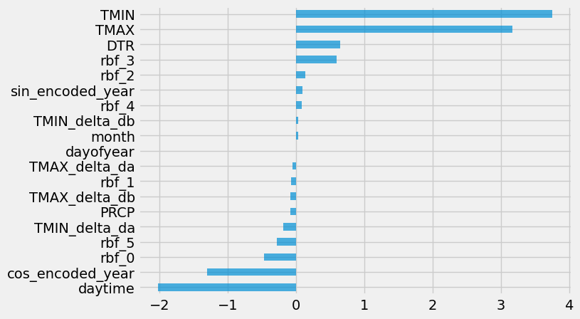
drop_features = ["dayofyear", "month", "TMIN_delta_db"]
X_train.drop(drop_features, axis=1, inplace=True)
X_test.drop(drop_features, axis=1, inplace=True)
X.drop(drop_features, axis=1, inplace=True)
for f in drop_features:
    features.remove(f)
DecisionTreeRegressor
Let’s explore the Decision Tree Regressor, a non-linear regression model:
dtr = DecisionTreeRegressor(random_state=RS)
dtr.fit(X_train, y_train)
y_pred = dtr.predict(X_test)
evaluate(y_test, y_pred)
Mean absolute error : 0.9473, Mean squared error : 1.2625
Next, we experiment with different tree depths ranging from 2 to 20. For each depth, we evaluate the model’s performance on both the training and testing data, recording the MAE scores for each.
mae_train_score = []
mae_test_score = []
for md in range(2, 21):
    dtr = DecisionTreeRegressor(max_depth=md, random_state=RS)
    dtr.fit(X_train, y_train)

    y_pred = dtr.predict(X_train)
    d_train = evaluate(y_train, y_pred, return_score=True)
    mae_train_score.append(d_train["mae"])

    y_pred = dtr.predict(X_test)
    d_test = evaluate(y_test, y_pred, return_score=True)
    mae_test_score.append(d_test["mae"])
plt.figure(figsize=(7, 5))
_ = plt.plot(range(2, 21), mae_train_score)
_ = plt.plot(range(2, 21), mae_test_score)
ax = plt.gca()
_ = ax.legend(["train", "test"])
_ = ax.set(title="Train/test error vs max_depth", xlabel="max_depth", ylabel="MAE")
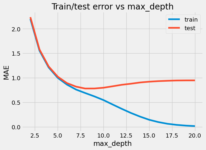
It seems like max_depth=8 is the best one:
dtr = DecisionTreeRegressor(max_depth=8, random_state=RS)
dtr.fit(X_train, y_train)
y_pred = dtr.predict(X_test)
results = pd.concat(
    [
        results,
        pd.Series(evaluate(y_test, y_pred, return_score=True))
        .to_frame("decision tree")
        .T,
    ],
    axis=0,
)
results
| mae | rmse | |
|---|---|---|
| baseline | 0.916753 | 1.214852 |
| ridge | 0.740136 | 0.984712 |
| decision tree | 0.782112 | 1.049301 |
Now we analyze feature importance and remove some useless features from the dataset:
fi = pd.DataFrame(data={"importance": dtr.feature_importances_}, index=X_train.columns)
fi.sort_values(by="importance", ascending=False, inplace=True)
ax = fi[:30].plot.barh(figsize=(7, 5), logx=True, alpha=0.7, legend=False)
ax.invert_yaxis()
_ = ax.set(
    title="Decision tree feature importance",
    xlabel="Importance (Log scale)",
    ylabel="Feature",
)
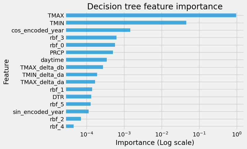
drop_features = ["rbf_2", "rbf_4", "sin_encoded_year"]
X_train.drop(drop_features, axis=1, inplace=True)
X_test.drop(drop_features, axis=1, inplace=True)
X.drop(drop_features, axis=1, inplace=True)
for f in drop_features:
    features.remove(f)
RandomForestRegressor
From scikit-learn’s documentation:
A random forest is a meta estimator that fits a number of classifying decision trees on various sub-samples of the dataset and uses averaging to improve the predictive accuracy and control over-fitting.
rfr = RandomForestRegressor(
    n_estimators=250,
    max_depth=13,
    min_samples_split=10,
    max_features=0.9,
    n_jobs=12,
    random_state=RS,
)
rfr.fit(X_train, y_train)
y_pred = rfr.predict(X_test)
evaluate(y_test, y_pred)
Mean absolute error : 0.6746, Mean squared error : 0.9102
results = pd.concat(
    [
        results,
        pd.Series(evaluate(y_test, y_pred, return_score=True))
        .to_frame("random forest")
        .T,
    ],
    axis=0,
)
results
| mae | rmse | |
|---|---|---|
| baseline | 0.916753 | 1.214852 |
| ridge | 0.740136 | 0.984712 |
| decision tree | 0.782112 | 1.049301 |
| random forest | 0.674629 | 0.910177 |
fi = pd.DataFrame(data={"importance": rfr.feature_importances_}, index=X_train.columns)
fi.sort_values(by="importance", ascending=False, inplace=True)
ax = fi[:25].plot.barh(figsize=(7, 5), logx=True, alpha=0.6, legend=False)
ax.invert_yaxis()
_ = ax.set(
    title="Random forest feature importance",
    xlabel="Importance (Log scale)",
    ylabel="Feature",
)
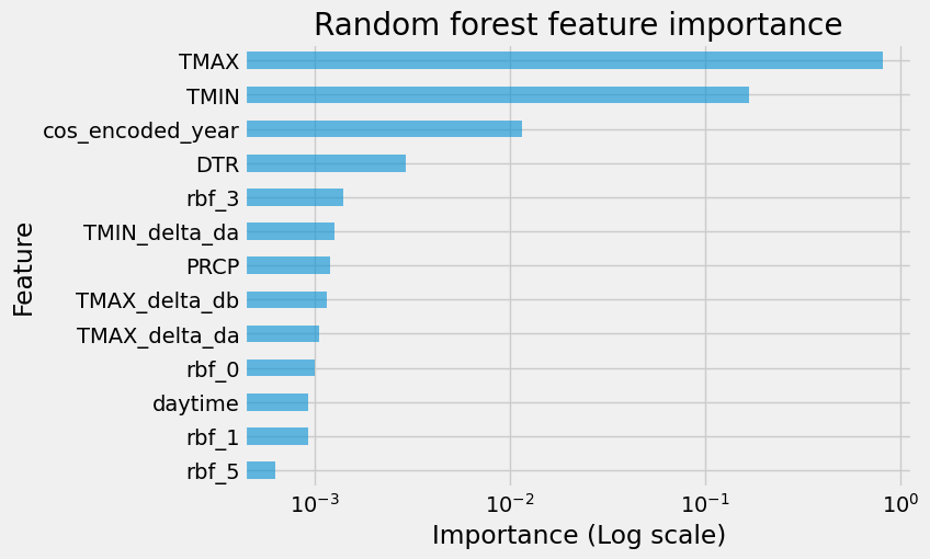
drop_features = ["rbf_5", "rbf_1"]
X_train.drop(drop_features, axis=1, inplace=True)
X_test.drop(drop_features, axis=1, inplace=True)
X.drop(drop_features, axis=1, inplace=True)
for f in drop_features:
    features.remove(f)
HistGradientBoostingRegressor
Next we use the HistGradientBoostingRegressor, a gradient boosting algorithm that’s known for its efficiency and performance:
hgbr = HistGradientBoostingRegressor(random_state=RS)
hgbr.fit(X_train, y_train)
y_pred = hgbr.predict(X_test)
evaluate(y_test, y_pred)
Mean absolute error : 0.6692, Mean squared error : 0.9037
results = pd.concat(
    [
        results,
        pd.Series(evaluate(y_test, y_pred, return_score=True))
        .to_frame("hist gradient boosting")
        .T,
    ],
    axis=0,
)
results
| mae | rmse | |
|---|---|---|
| baseline | 0.916753 | 1.214852 |
| ridge | 0.740136 | 0.984712 |
| decision tree | 0.782112 | 1.049301 |
| random forest | 0.674629 | 0.910177 |
| hist gradient boosting | 0.669222 | 0.903695 |
The default values are giving good results, but let’s try to perfom some hyperparameter optimization with Optuna. The optimization process aims to find the best combination of hyperparameters that results in a model with improved predictive performance.
FIXED_PARAMS = {}
FIXED_PARAMS["loss"] = "squared_error"
FIXED_PARAMS["monotonic_cst"] = {"TMIN": 1, "TMAX": 1}
FIXED_PARAMS["validation_fraction"] = 0.15
FIXED_PARAMS["n_iter_no_change"] = 15
FIXED_PARAMS["early_stopping"] = True
FIXED_PARAMS["random_state"] = RS


class Objective(object):
    def __init__(self, X, y, fixed_params=FIXED_PARAMS):
        self.X = X
        self.y = y
        self.fixed_params = fixed_params

    def __call__(self, trial):
        learning_rate = trial.suggest_float("learning_rate", 0.02, 0.2, log=True)
        max_iter = trial.suggest_categorical("max_iter", [50, 100, 150, 200, 250])
        max_leaf_nodes = trial.suggest_categorical(
            "max_leaf_nodes", [21, 26, 31, 36, 41]
        )
        max_depth = trial.suggest_int("max_depth", 6, 32, log=False)
        min_samples_leaf = trial.suggest_categorical(
            "min_samples_leaf", [10, 15, 20, 25, 30]
        )
        l2_regularization = trial.suggest_float(
            "l2_regularization", 1e-8, 1e-1, log=True
        )
        max_bins = trial.suggest_categorical("max_bins", [205, 225, 255])

        hgbr = HistGradientBoostingRegressor(
            learning_rate=learning_rate,
            max_iter=max_iter,
            max_leaf_nodes=max_leaf_nodes,
            max_depth=max_depth,
            min_samples_leaf=min_samples_leaf,
            l2_regularization=l2_regularization,
            max_bins=max_bins,
            **self.fixed_params
        )

        score = cross_val_score(
            hgbr, self.X, self.y, n_jobs=3, cv=3, scoring="neg_mean_absolute_error"
        )
        mae = -1.0 * score.mean()
        return mae
objective = Objective(X_train, y_train)

sampler = NSGAIISampler(
    population_size=100,
    seed=RS,
)
study = create_study(direction="minimize", sampler=sampler)
study.optimize(
    objective,
    n_trials=1000,
    n_jobs=1,
)
[I 2023-09-06 13:52:45,182] A new study created in memory with name: no-name-d32e6de4-7cae-43d5-8f5e-afe0d72605b9
[I 2023-09-06 13:52:45,989] Trial 0 finished with value: 1.8808348240559607 and parameters: {'learning_rate': 0.025532591774822706, 'max_iter': 50, 'max_leaf_nodes': 36, 'max_depth': 9, 'min_samples_leaf': 15, 'l2_regularization': 0.0012473085120470293, 'max_bins': 225}. Best is trial 0 with value:
...
[I 2023-09-06 14:01:29,745] Trial 999 finished with value: 0.6788856968370406 and parameters: {'learning_rate': 0.04112414787841993, 'max_iter': 250, 'max_leaf_nodes': 36, 'max_depth': 22, 'min_samples_leaf': 30, 'l2_regularization': 0.0024433893814918765, 'max_bins': 225}. Best is trial 868 with value: 0.6764808748435326.
hp = study.best_params.copy()
hp.update(FIXED_PARAMS)
for key, value in hp.items():
    print(f"{key:>20s} : {value}")
print(f"{'best objective value':>20s} : {study.best_value}")
       learning_rate : 0.04403581826578526
            max_iter : 200
      max_leaf_nodes : 36
           max_depth : 28
    min_samples_leaf : 25
   l2_regularization : 0.017899518645399605
            max_bins : 255
                loss : squared_error
       monotonic_cst : {'TMIN': 1, 'TMAX': 1}
 validation_fraction : 0.15
    n_iter_no_change : 15
      early_stopping : True
        random_state : 124
best objective value : 0.6764808748435326
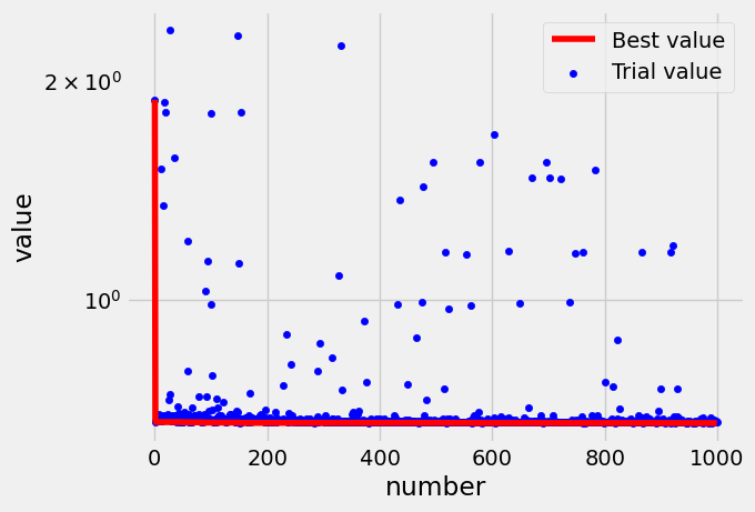
Next we plot the HPO history. We can observe that the minimization process is rapidly reaching a plateau:
trials = study.trials_dataframe()
score = np.ndarray(len(trials), dtype=np.float64)
i = 0
value_min = 1.0e15
for row in trials.itertuples():
    value_min = np.amin([value_min, row.value])
    score[row.number] = value_min
    i += 1
trials["best_value"] = score
ax = trials[["number", "best_value"]].plot(
    x="number", y="best_value", logy=True, color="r", label="Best value"
)
ax = trials[["number", "value"]].plot.scatter(
    x="number", y="value", logy=True, color="b", ax=ax, label="Trial value"
)
Let’s evaluate our model. Eval on train set:
n_splits = 3
kf = KFold(n_splits=n_splits, random_state=RS, shuffle=True)
y_pred = np.zeros_like(y_train)
hgbrs = []
for train_index, test_index in kf.split(X_train):
    hgbr = HistGradientBoostingRegressor(**hp)
    hgbr.fit(X_train.iloc[train_index], y_train.iloc[train_index])
    hgbrs.append(hgbr)
    y_pred[test_index] = hgbr.predict(X_train.iloc[test_index])
evaluate(y_train, y_pred)
Mean absolute error : 0.6767, Mean squared error : 0.9047
Eval on test set:
y_pred = np.zeros((X_test.shape[0],), dtype=np.float64)
for model in hgbrs:
    y_pred += model.predict(X_test)
y_pred /= len(hgbrs)
evaluate(y_test, y_pred)
Mean absolute error : 0.6673, Mean squared error : 0.9018
results = pd.concat(
    [
        results,
        pd.Series(evaluate(y_test, y_pred, return_score=True))
        .to_frame("hist gradient boosting w HPO")
        .T,
    ],
    axis=0,
)
results
| mae | rmse | |
|---|---|---|
| baseline | 0.916753 | 1.214852 |
| ridge | 0.740136 | 0.984712 |
| decision tree | 0.782112 | 1.049301 |
| random forest | 0.674629 | 0.910177 |
| hist gradient boosting | 0.669222 | 0.903695 |
| hist gradient boosting w HPO | 0.667300 | 0.901843 |
The final evaluation confirms that our HPO did not really improve the model. It does not always lead to better results…
Fill the missing TAVG values
Low it’s time to handle the missing TAVG values through prediction and imputation, ensuring that the dataset is ready for further analysis:
X_mv = df[df.TAVG.isna()][features]  # dataset with missing TAVG values
y_pred = np.zeros((X_mv.shape[0],), dtype=np.float64)
for model in hgbrs:
    y_pred += model.predict(X_mv)
y_pred /= len(hgbrs)
TAVG_pred = pd.DataFrame(data=y_pred, index=X_mv.index, columns=["TAVG_pred"])
df = pd.concat((df, TAVG_pred), axis=1)
df.TAVG = df.TAVG.fillna(df.TAVG_pred)
df.drop("TAVG_pred", axis=1, inplace=True)
df = df[["PRCP", "TAVG", "TMIN", "TMAX"]]
_ = msno.matrix(df)

Let’s save the updated dataset in our favorite file format:
df.to_parquet("./lyon_historical_temperatures.parquet")
In the following section we perform an analysis of the temperature anomalies during meteorological summer months with respect to a historical average. This will make use of the reconstructed variable TAVG, by taking the average of this mean daily temperature over the 3 warmest months of the year.
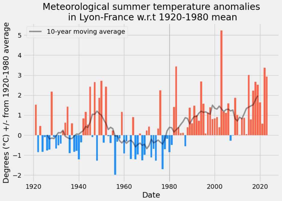
Meteorological Summer months temperature anomalies
We are going to analyzing temperature anomalies during meteorological summer months (June, July, August) in Lyon – Saint-Exupéry Airport, France, compared to a historical average:
start, end = "1920", "1980"

df_summer = T_month.loc[T_month.month.isin([6, 7, 8])].TAVG.resample("Y").mean()
t_summer = df_summer[start:end].mean()

anomaly = (df_summer - t_summer).copy(deep=True).to_frame("anomaly")
anomaly["label"] = anomaly.index.year.astype(str)
anomaly.loc[anomaly["label"].str[-1] != "0", "label"] = ""
rw = anomaly.anomaly.rolling(10, center=True).mean().to_frame("window")

fig, ax = plt.subplots(figsize=FS)
mask = anomaly[start:].anomaly > 0
colors = np.array(["dodgerblue"] * len(anomaly[start:]))
colors[mask.values] = "tomato"
plt.bar(anomaly[start:].index.year, anomaly[start:].anomaly, color=colors)
plt.plot(
    rw[start:].index.year.tolist(),
    rw[start:].window.values,
    "k",
    linewidth=3,
    alpha=0.4,
    label="10-year moving average",
)

_ = plt.axvline(x=int(end), color="grey", linewidth=1, alpha=0.5)
ax.legend()
ax.set_xlabel("Date")
ax.set_ylabel(f"Degrees (°C) +/- from {start}-{end} average")
ax.set_title(
    f"Meteorological summer temperature anomalies\n in Lyon – Saint-Exupéry Airport – France \nw.r.t {start}-{end} mean"
);
Reference
[1] Bernhardt, J., “A comparison of daily temperature-averaging methods: Uncertainties, spatial variability, and societal implications”, PhDT, Pennsylvania State University, 2016.