Lyon's Digital Terrain Model with IGN Data
In this post, we explore how to extract and merge data from a french high-resolution Digital Terrain Model (DTM). This DTM is provided by the IGN (National Institute of Geographic and Forest Information). It gives a detailed grid-based depiction of the topography of the entire French territory on a large scale. For our purposes, we will be working with the 5-meter resolution option, although a 1-meter resolution is also available. It can be found on this web page : https://geoservices.ign.fr/rgealti.
In the following we merge all the small files to generate a comprehensive raster. While this facilitates batch processing, it’s important to note that the memory usage might be substantial. Here are the steps followed:
- HTML Parsing with BeautifulSoup
- Data Organization with Pandas
- Bounding Box Definition
- Intersected “Department” Zones List
- Data Download
- Conversion to GeoTIFF Format
- Raster Mosaic
- Raster Bounding Box Cropping
- Point Queries
System and package versions
OS and package versions:
Python version       : 3.11.6
OS                   : Linux
Machine              : x86_64


contextily           : 1.4.0
geopandas            : 0.14.1
matplotlib           : 3.8.2
numpy                : 1.26.2
pandas               : 2.1.3
py7zr                : 0.20.6
pyproj               : 3.6.1
rasterio             : 1.3.9
requests             : 2.31.0
bs4                  : 4.12.2
osgeo                : 3.7.3
shapely              : 2.0.2
tqdm                 : 4.66.1
Python imports
import glob
import os
import re

import contextily as cx
import geopandas as gpd
import matplotlib.pyplot as plt
import numpy as np
import pandas as pd
import py7zr
import pyproj
import rasterio as rio
import requests
from bs4 import BeautifulSoup
from osgeo import gdal, osr
from rasterio.enums import Resampling
from rasterio.mask import mask
from rasterio.merge import merge
from rasterio.plot import show
from shapely.geometry import Point, Polygon
from shapely.ops import transform
from tqdm import tqdm

DATA_DIR_PATH = "/home/francois/Data/RGE_ALTI/5M/"
IGN_URL = "https://geoservices.ign.fr/rgealti"
DEPS_SHP_FP = "/home/francois/Data/RGE_ALTI/departements-20140306-50m-shp/departements-20140306-50m.shp"

tif_dir_path = os.path.join(DATA_DIR_PATH, "tif_files")
Parse the HTML from the IGN web page using BeautifulSoup
We specifically target and extract download links related to the 5-meter resolution, filtering out any links associated with the 1-meter resolution.
# Retrieve HTML content from IGN web page
response = requests.get(IGN_URL)

# Extract download links using BeautifulSoup
download_links = None
if response.status_code == 200:
    html_content = response.text
    soup = BeautifulSoup(html_content, "html.parser")
    pattern = re.compile(
        r"https://wxs\.ign\.fr/[^/]+/telechargement/prepackage/RGEALTI-5M_PACK_[^$]+\$[^/]+/file/[^/]+\.7z"
    )
    links = soup.find_all("a", href=pattern)
    download_links = [link["href"] for link in links]
else:
    print(f"Failed to retrieve the page. Status code: {response.status_code}")

# Display the number of download links found
if download_links:
    link_count = len(download_links)
else:
    link_count = 0
print(f"Found {link_count} download link(s)")
Found 105 download link(s)
Each download link is linked to its respective French “department” code.
Organize Data with Pandas
# Create Pandas DataFrame with download links
df = pd.DataFrame(data={"download_link": download_links})
df["compressed_file_name"] = df["download_link"].map(os.path.basename)
# Extract components and assert data integrity

def extract_components(s):
    base_name = s.split(".7z")[0]
    keys = ["dataset", "version", "res", "filetype", "crs", "dep", "date"]
    d = dict(zip(keys, base_name.split("_")))
    return pd.Series(d)


df[["dataset", "version", "res", "filetype", "crs", "dep", "date"]] = df[
    "compressed_file_name"
].apply(extract_components)
assert np.array_equal(df["dataset"].unique(), np.array(["RGEALTI"]))
assert np.array_equal(df["res"].unique(), np.array(["5M"]))
assert np.array_equal(df["filetype"].unique(), np.array(["ASC"]))
# Extract department codes and refine DataFrame

def get_dep_code(s):
    dep_code = s.removeprefix("D")
    if dep_code[0] == "0":
        dep_code = dep_code.removeprefix("0")
    return dep_code


df["dep_code"] = df["dep"].map(get_dep_code)
df = df.drop(["dataset", "version", "res", "dep", "filetype", "date"], axis=1)
df.head(3)
| download_link | compressed_file_name | crs | dep_code | |
|---|---|---|---|---|
| 0 | https://wxs.ign.fr/9u5z4x13jqu05fb3o9cux5e1/te... | RGEALTI_2-0_5M_ASC_LAMB93-IGN69_D001_2023-08-0... | LAMB93-IGN69 | 01 |
| 1 | https://wxs.ign.fr/9u5z4x13jqu05fb3o9cux5e1/te... | RGEALTI_2-0_5M_ASC_LAMB93-IGN69_D002_2020-09-0... | LAMB93-IGN69 | 02 |
| 2 | https://wxs.ign.fr/9u5z4x13jqu05fb3o9cux5e1/te... | RGEALTI_2-0_5M_ASC_LAMB93-IGN69_D003_2023-08-1... | LAMB93-IGN69 | 03 |
Note that the Coordinate Reference System (CRS) is always Lambert-93 or EPSG:2154 for this data when dealing with regions in European France.
Bounding box definition
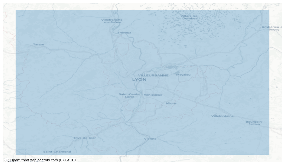
The first step involves defining a bounding box that encapsulates the region of interest: Lyon, france.
# Define bounding box coordinates in EPSG:4326
bbox = (4.346466, 45.463020, 5.340729, 46.030342)

# Define points to create a polygon
point1 = (bbox[0], bbox[1])
point2 = (bbox[0], bbox[3])
point3 = (bbox[2], bbox[3])
point4 = (bbox[2], bbox[1])
# Create a polygon from the points
polygon = Polygon([point1, point2, point3, point4])

# Display the polygon
polygon

# display the polygon with map tiles
bbox_gdf = gpd.GeoSeries([polygon], crs="EPSG:4326")
fig, ax = plt.subplots(1, figsize=(12, 12))
ax = bbox_gdf.plot(alpha=0.3, ax=ax)
cx.add_basemap(ax, crs=bbox_gdf.crs.to_string(), source=cx.providers.CartoDB.Positron)
ax.set_axis_off()
Intersected “Department” zones list
To determine which French departments intersect with our defined bounding box, we use a shapefile containing the polygons of French department zones expressed in EPSG:4326 coordinates. The shapefile was downloaded from this page, specifically the Export de mars 2014 - vérifié et simplifié à 50m
zones = gpd.read_file(DEPS_SHP_FP)[["code_insee", "geometry"]]
zones.head(2)
| code_insee | geometry | |
|---|---|---|
| 0 | 01 | POLYGON ((5.25559 45.78459, 5.23987 45.77758, ... |
| 1 | 02 | POLYGON ((3.48175 48.86640, 3.48647 48.85768, ... |
We can now identify which department zones intersect with the previously defined bounding box.
intersected_zones = zones.loc[zones.intersects(polygon)]
intersected_zones
| code_insee | geometry | |
|---|---|---|
| 0 | 01 | POLYGON ((5.25559 45.78459, 5.23987 45.77758, ... |
| 38 | 38 | POLYGON ((5.44781 45.07178, 5.44982 45.07078, ... |
| 42 | 42 | POLYGON ((4.02072 45.32827, 4.01866 45.32764, ... |
| 69 | 69 | POLYGON ((4.87189 45.52749, 4.86173 45.51689, ... |
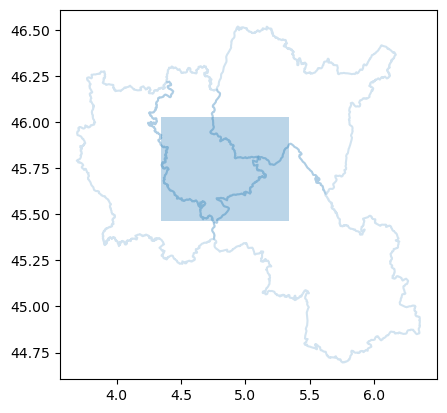
We visualize these intersected zones along with the bounding box.
ax = intersected_zones.boundary.plot(alpha=0.2, label="insee_code")
ax = bbox_gdf.plot(alpha=0.3, ax=ax)
Finally, we obtain the list of French department codes that intersect with the bounding box.
zone_codes = intersected_zones.code_insee.values.tolist()
zone_codes
['01', '38', '42', '69']
IGN data download
Now that we have identified the French department codes intersecting with the bounding box, let’s proceed with downloading and organizing the relevant DTM data.
# Create a list of download items for the intersected zones
download_items = []
for zone_code in zone_codes:
    download_items.append(
        df.loc[
            df.dep_code == zone_code,
            ["download_link", "compressed_file_name", "crs"],
        ].to_dict(orient="records")[0]
    )
Next, we iterate through the download items, downloading and uncompressing the relevant data.
# List to store paths of downloaded and uncompressed files
dem_dir_paths = []

# Iterate through download items
for download_item in download_items:
    crs = download_item["crs"]

    # Define file paths
    dem_file_url = download_item["download_link"]
    dem_file_name = download_item["compressed_file_name"]
    dem_file_path = os.path.join(DATA_DIR_PATH, dem_file_name)
    dem_dir_path = os.path.splitext(dem_file_path)[0]

    # Download file if not already downloaded
    is_downloaded = os.path.isfile(dem_file_path) | os.path.isdir(dem_dir_path)
    if not is_downloaded:
        print(f"downloading file {dem_file_name}")
        r = requests.get(dem_file_url, stream=True)
        with open(dem_file_path, "wb") as fd:
            for chunk in r.iter_content(chunk_size=512):
                fd.write(chunk)

    # Uncompress file if not already uncompressed
    dem_dir_paths.append(dem_dir_path)
    is_uncompressed = os.path.isdir(dem_dir_path)
    if not is_uncompressed:
        print(f"uncompressing file {dem_file_name}")
        with py7zr.SevenZipFile(dem_file_path, "r") as archive:
            archive.extractall(path=DATA_DIR_PATH)
        if os.path.exists(dem_file_path):
            os.remove(dem_file_path)
The dem_dir_paths list now contains the paths of the downloaded and uncompressed files:
dem_dir_paths
['/home/francois/Data/RGE_ALTI/5M/RGEALTI_2-0_5M_ASC_LAMB93-IGN69_D001_2023-08-08',
 '/home/francois/Data/RGE_ALTI/5M/RGEALTI_2-0_5M_ASC_LAMB93-IGN69_D038_2020-11-13',
 '/home/francois/Data/RGE_ALTI/5M/RGEALTI_2-0_5M_ASC_LAMB93-IGN69_D042_2023-08-10',
 '/home/francois/Data/RGE_ALTI/5M/RGEALTI_2-0_5M_ASC_LAMB93-IGN69_D069_2023-08-10']
These directories contain the DTM data for the specified French departments, and we can proceed with the data conversion.
Convert .asc files to .tif files
The next step is to convert the .asc files to .tif files for compatibility with various geospatial tools and libraries.
# Create a directory to store the tif files if it doesn't exist
if not os.path.exists(tif_dir_path):
    os.makedirs(tif_dir_path)
    print(f"tif files directory : {tif_dir_path}")
The following functions and class, extracted from Guillaume Attard’s great blog post [1], are used to handle the conversion from .asc to .tif.
def get_header_asc(filepath):
    """Function to read the header of an asc file and return the data as a dictionary.
    """
    file = open(filepath)
    content = file.readlines()[:6]
    content = [item.split() for item in content]
    return dict(content)


class RGEitem:
    """Class to handle RGE items.
    """

    def __init__(self, filepath):
        self.filename = os.path.basename(filepath)
        self.dir = os.path.dirname(filepath)
        self.data = np.loadtxt(filepath, skiprows=6)
        self.header = get_header_asc(filepath)
        self.ncols = int(self.header["ncols"])
        self.nrows = int(self.header["nrows"])
        self.xllc = float(self.header["xllcorner"])
        self.yllc = float(self.header["yllcorner"])
        self.res = float(self.header["cellsize"])
        self.zmin = float(self.data.min())
        self.zmax = float(self.data.max())
        self.novalue = -99999.0


def asc_to_tif(file, output_rasterpath, epsg):
    """Function to transform an .asc file into a geoTIFF
    """
    xmin = file.xllc
    ymax = file.yllc + file.nrows * file.res
    geotransform = (xmin, file.res, 0, ymax, 0, -file.res)

    # Open the file
    output_raster = gdal.GetDriverByName("GTiff").Create(
        output_rasterpath, file.ncols, file.nrows, 1, gdal.GDT_Float32
    )
    # Specify the coordinates.
    output_raster.SetGeoTransform(geotransform)
    # Establish the coordinate encoding.
    srs = osr.SpatialReference()
    # Specify the projection.
    srs.ImportFromEPSG(epsg)
    # Export the coordinate system to the file.
    output_raster.SetProjection(srs.ExportToWkt())
    # Writes the array.
    output_raster.GetRasterBand(1).WriteArray(file.data)
    # Set nodata value.
    output_raster.GetRasterBand(1).SetNoDataValue(file.novalue)
    output_raster.FlushCache()
Now, we find all .asc files in the downloaded directories and convert them to .tif.
# Function to find all asc files in a directory
def find_asc_files(directory):
    directory = os.path.join(directory, "**/*.asc")
    asc_file_paths = glob.glob(directory, recursive=True)
    return asc_file_paths

# List to store paths of all converted tif files
all_tif_file_paths = []

# Iterate through the downloaded directories
for dem_dir_path in dem_dir_paths:
    print(f"top directory : {dem_dir_path}")
    asc_file_paths = find_asc_files(dem_dir_path)
    asc_file_count = len(asc_file_paths)
    print(f"{asc_file_count} asc files")
    for asc_file_path in tqdm(asc_file_paths):
        asc_file_name = os.path.basename(asc_file_path)
        asc_file_name, asc_file_extension = os.path.splitext(
            os.path.basename(asc_file_name)
        )
        tif_file_path = os.path.join(tif_dir_path, asc_file_name + ".tif")
        all_tif_file_paths.append(tif_file_path)
        if not os.path.isfile(tif_file_path):
            file = RGEitem(asc_file_path)
            asc_to_tif(file, tif_file_path, epsg=2154)
top directory : /home/francois/Data/RGE_ALTI/5M/RGEALTI_2-0_5M_ASC_LAMB93-IGN69_D001_2023-08-08
291 asc files

top directory : /home/francois/Data/RGE_ALTI/5M/RGEALTI_2-0_5M_ASC_LAMB93-IGN69_D038_2020-11-13
383 asc files

top directory : /home/francois/Data/RGE_ALTI/5M/RGEALTI_2-0_5M_ASC_LAMB93-IGN69_D042_2023-08-10
248 asc files

top directory : /home/francois/Data/RGE_ALTI/5M/RGEALTI_2-0_5M_ASC_LAMB93-IGN69_D069_2023-08-10
174 asc files
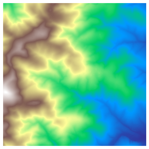
Here is an example of one of these small .tif files:
fig, ax = plt.subplots(1, figsize=(6, 6))

with rio.open(tif_file_path) as img:
    show(img, cmap="terrain", ax=ax)

ax.set_axis_off()
The total number of converted .tif files is:
len(all_tif_file_paths)
1096
Raster Mosaic with Python
The next step is to create a raster mosaic from these individual tiles.
# Define the path for the output mosaic
output_mosaic_path = os.path.join(tif_dir_path, "lyon_mosaic.tif")

# List to store raster objects for mosaic
raster_to_mosaic = []
for p in all_tif_file_paths:
    raster = rio.open(p)
    raster_to_mosaic.append(raster)
We use the merge function from rasterio to create the mosaic:
mosaic, output = merge(raster_to_mosaic)
Update the metadata for the output mosaic:
output_meta = raster.meta.copy()
output_meta.update(
    {
        "driver": "GTiff",
        "height": mosaic.shape[1],
        "width": mosaic.shape[2],
        "transform": output,
    }
)
Write the mosaic to a new GeoTIFF file:
with rio.open(output_mosaic_path, "w", **output_meta) as m:
    m.write(mosaic)

del mosaic
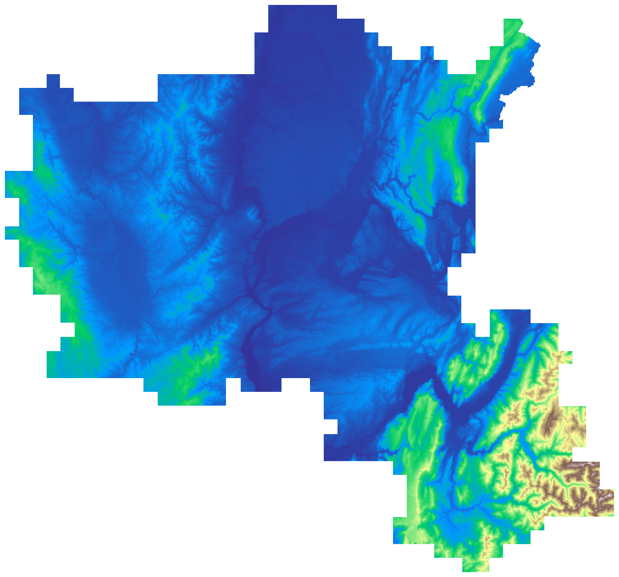
Now, let’s downsample this mosaic in order to save some memory space, and plot it:
upscale_factor = 0.125

with rio.open(output_mosaic_path) as dataset:
    # resample data to target shape
    data = dataset.read(
        out_shape=(
            dataset.count,
            int(dataset.height * upscale_factor),
            int(dataset.width * upscale_factor),
        ),
        resampling=Resampling.bilinear,
    )
    data = np.where(data == -99999.0, np.nan, data)
fig, ax = plt.subplots(1, figsize=(16, 16))

show(data, cmap="terrain", ax=ax)
ax.set_axis_off()
Raster Bounding Box Cropping with Rasterio
Now that we have our mosaic raster and a defined bounding box in the Lambert 93 (LAM93) projected CRS, let’s proceed with cropping the raster to the extent of our bounding box. Remember that the bounding box is expressed in EPSG:4326 while the raster is in EPSG:2154.
# Transform the bounding box polygon to the mosaic's CRS (Lambert 93)
wgs84 = pyproj.CRS("EPSG:4326")
lam93 = pyproj.CRS("EPSG:2154")
project = pyproj.Transformer.from_crs(wgs84, lam93, always_xy=True).transform
polygon_lam93 = transform(project, polygon)
polygon_lam93

# Open the mosaic raster
mosaic_raster = rio.open(output_mosaic_path)
# Check the CRS of the mosaic raster
mosaic_raster.crs
CRS.from_epsg(2154)
The CRS of the mosaic raster is confirmed to be EPSG:2154, which corresponds to Lambert 93. Now, let’s use Rasterio to crop the mosaic raster to the extent of the transformed bounding box:
# Crop the mosaic raster to the bounding box
out_image, out_transform = mask(mosaic_raster, [polygon_lam93], crop=True, filled=False)

out_meta = mosaic_raster.meta
out_meta.update(
    {
        "driver": "GTiff",
        "height": out_image.shape[1],
        "width": out_image.shape[2],
        "transform": out_transform,
    }
)
We’ve successfully cropped the mosaic raster to the extent of the defined bounding box. The resulting cropped raster is stored in out_image, and the associated metadata is stored in out_meta.
Save and plot
Now that we have successfully cropped the mosaic raster to the extent of our bounding box, let’s save the resulting raster and create a visual representation.
# Save the cropped raster to a new GeoTIFF file
with rio.open("lyon_dem.tif", "w", **out_meta) as dest:
    dest.write(out_image)
Now, let’s open the saved raster for visualization and analysis:
dem = rio.open("lyon_dem.tif")
# Plot the cropped raster
fig, ax = plt.subplots(1, figsize=(16, 16))
_ = show(dem, cmap="terrain", ax=ax)
ax.set_axis_off()
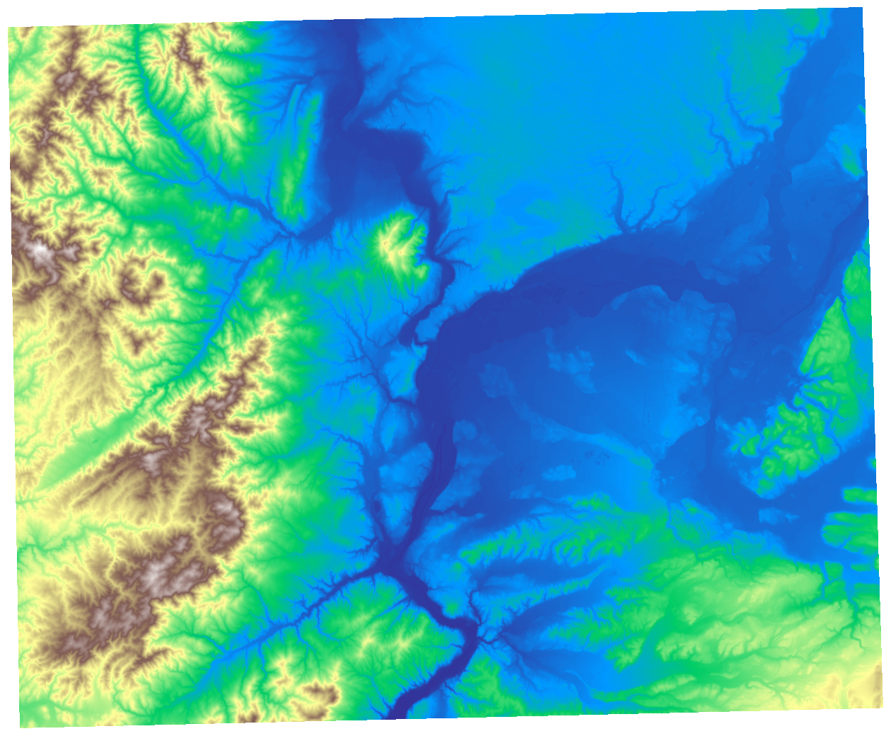
The resulting plot showcases the elevation data within the cropped region.
Point queries
In this section, we perform point queries on the cropped elevation data to extract elevation values at randomly generated coordinates within the region of interest.
rng = np.random.default_rng(421)
# Set the number of random coordinates you want
num_points = 1000

# Generate random x, y coordinates within the bounding box
random_x = rng.uniform(bbox[0], bbox[2], num_points)
random_y = rng.uniform(bbox[1], bbox[3], num_points)
point_coords = [transform(project, Point(x, y)) for x, y in zip(random_x, random_y)]
point_coords = [(p.x, p.y) for p in point_coords]

# Create a GeoDataFrame to store the random points
points = pd.DataFrame(point_coords, columns=["x_lam93", "y_lamb93"])
points["x_wgs84"] = random_x
points["y_wgs84"] = random_y
points_gdf = gpd.GeoDataFrame(
    points,
    geometry=gpd.points_from_xy(points.x_lam93, points.y_lamb93),
    crs="EPSG:2154",
)

# Plot the elevation map with sample points
fig, ax = plt.subplots(1, figsize=(10, 8))
figure = show(dem, cmap="terrain", ax=ax)
im = figure.get_images()[0]
clb = fig.colorbar(im, ax=ax)
clb.ax.set_title("Elevation (m)", fontsize=8)
ax = points_gdf.plot(ax=ax, c="k", markersize=3, alpha=0.4)
_ = plt.axis("off")
_ = ax.set(title="Elevation map of the region of Lyon, FR")
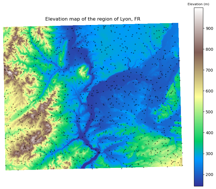
Now, let’s perform point queries to extract elevation values at these random points:
%%time
points["elevation"] = [x[0] for x in dem.sample(point_coords)]
points.loc[points["elevation"] < 0.0, "elevation"] = np.nan
points.head(3)
CPU times: user 15.8 ms, sys: 2.31 ms, total: 18.1 ms
Wall time: 17.2 ms
| x_lam93 | y_lamb93 | x_wgs84 | y_wgs84 | elevation | |
|---|---|---|---|---|---|
| 0 | 818322.302210 | 6.540550e+06 | 4.527680 | 45.954361 | 297.980011 |
| 1 | 820552.295444 | 6.510972e+06 | 4.548974 | 45.687670 | 709.400024 |
| 2 | 826049.449585 | 6.494117e+06 | 4.615158 | 45.534934 | 353.480011 |
The resulting GeoDataFrame points now includes the random points’ coordinates in both Lambert 93 (x_lam93, y_lamb93) and WGS84 (x_wgs84, y_wgs84) CRS, along with the corresponding elevation values.
print(points["elevation"].max(), points["elevation"].min())
839.79 150.5
References
[1] Guillaume Attard (2022) https://medium.com/@gui.attard/pre-processing-the-dem-of-france-rge-alti-5m-for-implementation-into-earth-engine-de9a0778e0d9