Finding the most concentrated areas of bakeries in Lyon
In this blog post, we’ll use Python to analyze the distribution of bakeries in Lyon, France. Our goal is to identify the areas with the highest concentration of bakeries in the city, potential hotspots for bread lovers. We will be using data from OpenStreetMap to achieve this.
Outline
- Imports
- Bounding box
- Fetch the data from Open Street Map
- Data cleanup
- Building a density surface
- The Bakery hotspots
Imports
Here we import the necessary libraries and modules that will help us fetch, process, and visualize the bakery data.
import contextily as cx
import matplotlib.pyplot as plt
import numpy as np
import osmnx as ox
import xyzservices.providers as xyz
from scipy.stats import gaussian_kde
from shapely import get_coordinates
from shapely.geometry import Polygon
from skimage.feature import peak_local_max

FS = (12, 12)  # figure size
KDE_FACTOR = 0.1  # kernel-density estimate factor
N_HOTSPOTS = 6  # fixed number of hotspots
Bounding box
We start by defining a bounding box encompassing the city of Lyon to query the points of interest from OpenStreetMap within this specific geographic area.
# A bounding box is a rectangular area defined by its minimum and maximum coordinates.
bbox = (4.78, 45.71, 4.92, 45.80)

# Extract coordinates for better readability
min_lon, min_lat, max_lon, max_lat = bbox

# Create points representing the corners of the bounding box
bottom_left = (min_lon, min_lat)
bottom_right = (max_lon, min_lat)
top_right = (max_lon, max_lat)
top_left = (min_lon, max_lat)

# Create a Shapely Polygon object from the bounding box coordinates
polygon = Polygon([bottom_left, bottom_right, top_right, top_left])
polygon

Fetch the data from Open Street Map
We use the osmnx library to fetch bakery data directly from OpenStreetMap. We’ll use the shop tag with a value of ‘bakery’ to filter for relevant locations.
%%time
tags = {"shop": "bakery"}
bakeries_gdf = ox.features.features_from_polygon(polygon, tags)
CPU times: user 43.2 ms, sys: 13 ms, total: 56.2 ms
Wall time: 70.8 ms
bakeries_gdf = bakeries_gdf.reset_index(drop=False)
bakeries_gdf.shape
(394, 123)
We successfully retrieved 394 rows. Each entry includes 123 data columns containing information from OpenStreetMap.
To ensure accurate spatial calculations and analysis, we reproject the bakeries GeoDataFrame from the original geographic coordinate system to the projected coordinate system: EPSG:2154.
bakeries_gdf = bakeries_gdf.to_crs("EPSG:2154")
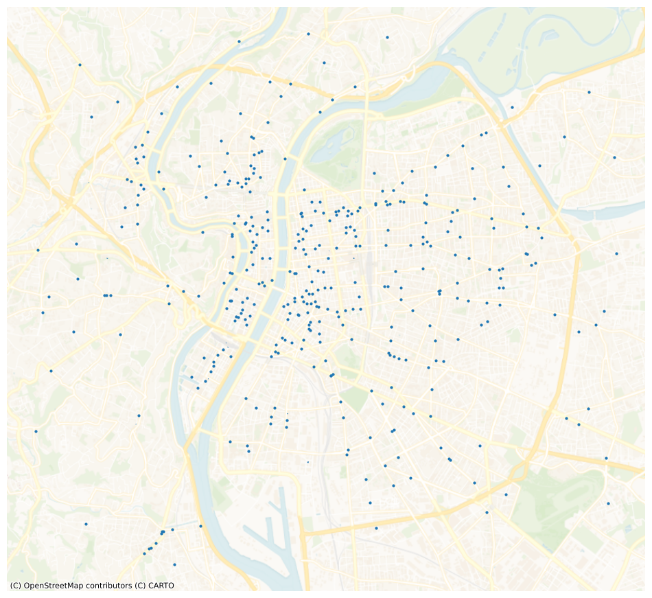
The following visualization depicts the raw distribution of bakeries (represented by blue markers) within the bounding box.
ax = bakeries_gdf.plot(markersize=4, figsize=FS)
cx.add_basemap(
    ax,
    source=xyz.CartoDB.VoyagerNoLabels,
    crs=bakeries_gdf.crs.to_string(),
    alpha=0.8,
)
_ = plt.axis("off")
Data cleanup
To focus on essential information, we filter the data to retain only points representing bakeries (excluding lines and polygons).
bakeries_gdf = bakeries_gdf.loc[bakeries_gdf.element_type == "node"]
The dataset contains a substantial number of columns, due to the rich metadata available from OpenStreetMap.
cols = bakeries_gdf.columns.to_list()
print(cols[:20])
print(f"column count : {len(cols)}")
['element_type', 'osmid', 'name', 'opening_hours', 'payment:cash', 'payment:credit_cards', 'phone', 'shop', 'wheelchair', 'geometry', 'access:covid19', 'opening_hours:covid19', 'payment:contactless', 'payment:visa', 'ref:FR:SIRET', 'fax', 'check_date', 'delivery:covid19', 'description:covid19', 'email']
column count : 123
We reduce the dataset to include solely the name and geometry columns, discarding unnecessary attributes.
bakeries_gdf = bakeries_gdf[["name", "geometry"]]
To maintain data integrity, we eliminate records lacking a name attribute, as these entries are likely incomplete and unreliable for our analysis.
bakeries_gdf.isna().sum(axis=0)
name        8
geometry    0
dtype: int64
bakeries_gdf = bakeries_gdf.dropna()
bakeries_gdf.shape
(372, 2)
The final dataset comprises 372 bakeries with their corresponding geographic coordinates, ready for further exploration.
bakeries_gdf.head(3)
| name | geometry | |
|---|---|---|
| 0 | Boulangerie Patisserie des Gratte Ciel | POINT (846015.870 6520210.859) |
| 1 | Boulangerie Pâtisserie Maison Champeaud | POINT (846751.582 6518543.900) |
| 2 | L'atelier de Xavier | POINT (845016.256 6515517.100) |
Let’s look for my personal favorite bakery, Partisan:
bakeries_gdf.loc[bakeries_gdf.name.str.contains("Partisan")]
| name | geometry | |
|---|---|---|
| 242 | Partisan Boulanger | POINT (842382.257 6521422.948) |
Building a density surface
To estimate the density function of bakery locations, we employ the Gaussian kernel density estimation (KDE) method provided by scipy.stats.gaussian_kde. This approach allows us to create a smooth 2D density function from the given point cloud data. The KDE method is particularly effective for visualizing the spatial distribution of bakery locations, and is allowing us to easily look for maxima.
We first extract the coordinates of the bakery locations and convert them into a numpy array:
points = np.array(get_coordinates(bakeries_gdf.geometry.values))
We then create a KDE object. Here we do not use the automatic bandwidth algorithms but give a scalar value to the bw_method argument, in order to control the bandwidth of the kernel, which affects the smoothness of the estimated density.
kde = gaussian_kde(points.T, bw_method=KDE_FACTOR)
Next, we define a grid over which we will evaluate the density. The grid is created using np.mgrid, which generates a mesh grid of points within the range of the input coordinates. Note that we give complex integer values for the step lengths:
if the step length is a complex number (e.g. 5j), then the integer part of its magnitude is interpreted as specifying the number of points to create between the start and stop values, where the stop value is inclusive.
x_min, x_max = points[:, 0].min(), points[:, 0].max()
y_min, y_max = points[:, 1].min(), points[:, 1].max()
x_grid, y_grid = np.mgrid[x_min:x_max:400j, y_min:y_max:400j]
positions = np.vstack([x_grid.ravel(), y_grid.ravel()])
We then evaluate the density at each point in the grid using the KDE object:
density = np.reshape(kde(positions).T, x_grid.shape).T
Finally, we find the location of the maximum density by identifying the indices of the maximum value in the density array. This gives us the coordinates of the point with the highest density of bakeries.
j_max, i_max = = np.unravel_index(np.argmax(density), density.shape)
x_max_density, y_max_density = x_grid[i_max, j_max], y_grid[i_max, j_max]
plt.figure(figsize=FS)
plt.imshow(density, extent=[x_min, x_max, y_min, y_max], origin="lower", cmap="YlOrBr")
ax = plt.gca()
ax = bakeries_gdf.plot(markersize=4, ax=ax, alpha=0.25)
plt.plot(x_max_density, y_max_density , marker="*", markersize=10, color="black")
cx.add_basemap(
    ax,
    source=xyz.CartoDB.Positron,
    crs=bakeries_gdf.crs.to_string(),
    alpha=0.6,
)
_ = plt.axis("off")
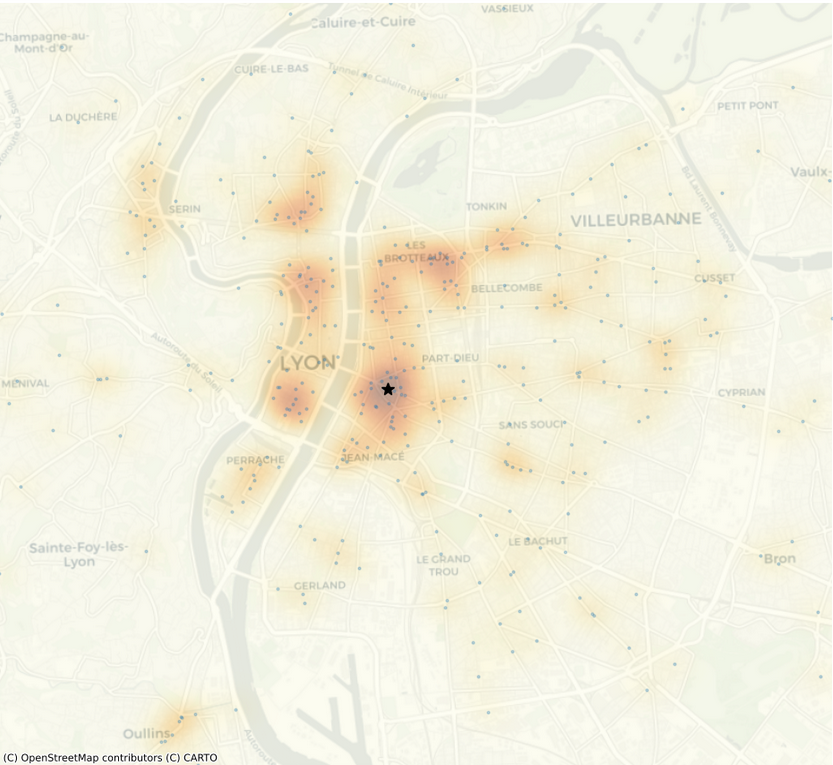
The maximum density of bakeries is found to be located between the Guillotière and Saxe-Gambetta districts.
The Bakery hotspots
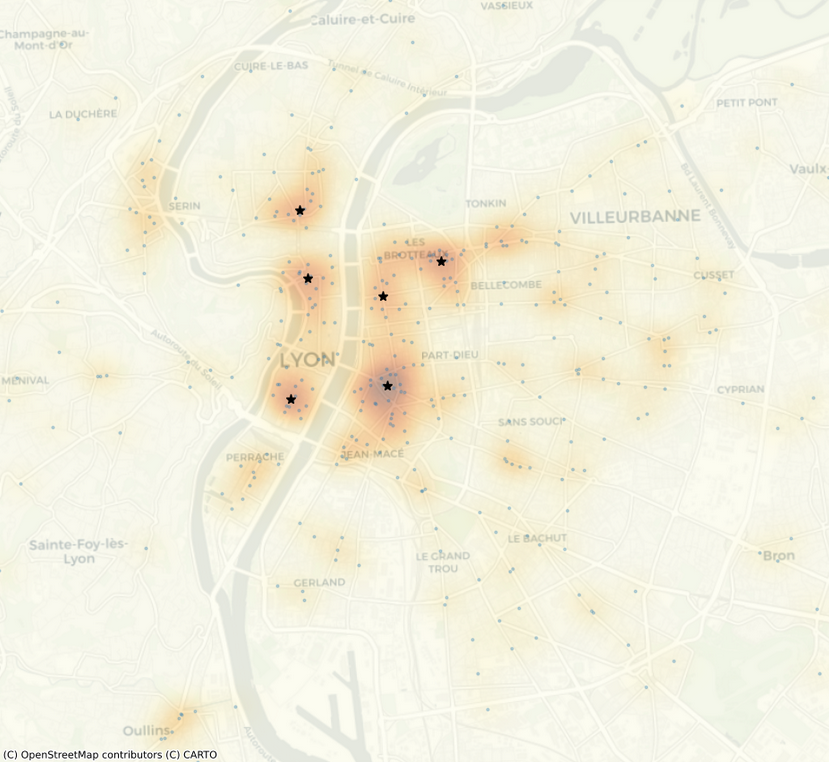
To identify the hotspots where bakeries are most densely concentrated, we use image local maxima detection and select the N_HOTSPOTS first values:
coordinates = peak_local_max(density, min_distance=1)

coords = []
for i in range(N_HOTSPOTS):
    j_max, i_max = coordinates[i, :]
    x, y = x_grid[i_max, j_max], y_grid[i_max, j_max]
    coords.append([x,y])
plt.figure(figsize=FS)
plt.imshow(density, extent=[x_min, x_max, y_min, y_max], origin="lower", cmap="YlOrBr")
ax = plt.gca()
ax = bakeries_gdf.plot(markersize=4, ax=ax, alpha=0.25)
for i in range(n_hotspots):
    plt.plot(coords[i][0], coords[i][1], marker="*", markersize=8, color="grey")
cx.add_basemap(
    ax,
    source=xyz.CartoDB.Positron,
    crs=bakeries_gdf.crs.to_string(),
    alpha=0.6,
)
_ = plt.axis("off")