Analyzing tramontane wind frequency
The tramontane wind, a defining feature of Pyrénées-Orientales region, is known for sweeping through the south of France with its characteristic force and direction from the northwest. Recently, I read studies suggesting that the tramontane’s frequency may be declining. Curious to explore this, I decided to look into open weather data provided by Météo France to examine changes in this wind since 1980.
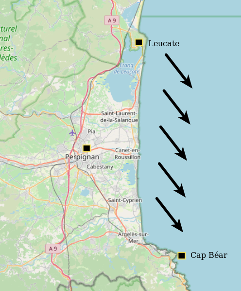
I’ll focus on three locations close to my heart: Cap Béar, Perpignan, and Leucate, which are well distributed along the Pyrénées-Orientales coast. Though Leucate lies just across the northern border in the Aude department, it remains closely connected to the region.
Outline
- Data source
- Imports and system
- Load and explore the data
- Cap Béar
- Perpignan
- Leucate
- Conclusion
- Citation
- Bonus : the 3, 6, 9 days rule
I should clarify that I am not an expert in atmospheric or climate science.
Data source
We begin by downloading four CSV files from the French open weather data website (https://meteo.data.gouv.fr/). These files are organized by two distinct periods and two regions:
- Time Periods: 1950-2022 and 2023-2024
- Regions (French departments): Pyrénées-Orientales (66) and Aude (11)
The CSV files are named as follows:
Q_66_previous-1950-2022_RR-T-Vent.csvQ_66_latest-2023-2024_RR-T-Vent.csvQ_11_previous-1950-2022_RR-T-Vent.csvQ_11_latest-2023-2024_RR-T-Vent.csv
To access these files on the site, follow these steps:
- Navigate to “Données climatologiques de base” (Basic Climate Data).
- Select “Données quotidiennes” (Daily Data).
- Choose either Pyrénées-Orientales (66) or Aude (11).
- Download data for the respective periods: 1950-2022 and 2023-2024.
Imports and system
The analysis is conducted in a Python 3.13.0 environment packaged by conda-forge on Linux. Below are the primary libraries used in the following:
import missingno as msno
import numpy as np
import pandas as pd
from scipy.optimize import curve_fit
from sklearn.linear_model import LinearRegression
from sklearn.preprocessing import PolynomialFeatures, RobustScaler
Package versions:
matplotlib :  3.9.2
missingno  :  0.5.2
numpy      :  2.1.2
pandas     :  2.2.3
sklearn    :  1.5.2
scipy      : 1.14.1
Load and explore the data
We begin by loading the datasets:
%%time
df_1 = pd.read_csv("./66/Q_66_previous-1950-2022_RR-T-Vent.csv", delimiter=";")
df_2 = pd.read_csv("./66/Q_66_latest-2023-2024_RR-T-Vent.csv", delimiter=";")
df_3 = pd.read_csv("./11/Q_11_previous-1950-2022_RR-T-Vent.csv", delimiter=";")
df_4 = pd.read_csv("./11/Q_11_latest-2023-2024_RR-T-Vent.csv", delimiter=";")
CPU times: user 2.33 s, sys: 688 ms, total: 3.02 s
Wall time: 3.06 s
Next, we combine all four datasets into one dataframe:
df_all = pd.concat((df_1, df_2, df_3, df_4), axis=0)
The NOM_USUEL column identifies the location, which allows us to filter for the specific sites of interest.
np.sort(df_all.NOM_USUEL.unique())[:5]
array(['ALAIGNE', 'AMELIE-LES-BAINS', 'ANGLES_LES', 'ANGOUSTRINE',
       'ARAGON'], dtype=object)
The locations we’re focusing on are CAP BEAR, PERPIGNAN and LEUCATE, so we filter the data accordingly:
df_all = df_all.loc[df_all.NOM_USUEL.isin(["CAP BEAR", "PERPIGNAN", "LEUCATE"])]
Let’s visualize the number of records by location:
ax = (
    df_all.groupby("NOM_USUEL")
    .size()
    .sort_values(ascending=False)
    .head(10)[::-1]
    .plot.barh(figsize=(6, 2), alpha=0.7)
)

We will see later that for Leucate, the data history is shorter, extending back only to 1995.
For context, here is a list of columns in the dataset:
df_all.columns
Index(['NUM_POSTE', 'NOM_USUEL', 'LAT', 'LON', 'ALTI', 'AAAAMMJJ', 'RR', 'QRR',
       'TN', 'QTN', 'HTN', 'QHTN', 'TX', 'QTX', 'HTX', 'QHTX', 'TM', 'QTM',
       'TNTXM', 'QTNTXM', 'TAMPLI', 'QTAMPLI', 'TNSOL', 'QTNSOL', 'TN50',
       'QTN50', 'DG', 'QDG', 'FFM', 'QFFM', 'FF2M', 'QFF2M', 'FXY', 'QFXY',
       'DXY', 'QDXY', 'HXY', 'QHXY', 'FXI', 'QFXI', 'DXI', 'QDXI', 'HXI',
       'QHXI', 'FXI2', 'QFXI2', 'DXI2', 'QDXI2', 'HXI2', 'QHXI2', 'FXI3S',
       'QFXI3S', 'DXI3S', 'QDXI3S', 'HXI3S', 'QHXI3S', 'DRR', 'QDRR'],
      dtype='object')
The columns prefixed with F relate to wind speed, D to wind direction, H to time, and Q to data quality. We select the following columns for our analysis:
NOM_USUEL: place nameAAAAMMJJ: date (YYYYMMDD)FXI: daily maximum of the peak hourly instantaneous wind force at 10 meters (in m/s and tenths)DXI: direction of FXI (in 360° compass rose format)
cols = ["NOM_USUEL", "AAAAMMJJ", "FXI", "DXI"]
df_all = df_all[cols]
df_all.head(3)
| NOM_USUEL | AAAAMMJJ | FXI | DXI | |
|---|---|---|---|---|
| 660298 | PERPIGNAN | 19500101 | 15.0 | NaN |
| 660299 | PERPIGNAN | 19500102 | 19.0 | NaN |
| 660300 | PERPIGNAN | 19500103 | 31.0 | NaN |
We remove rows with a missing value:
df_all = df_all.dropna(how="any")
We convert the date strings to a datetime index, for easier handling:
df_all["date"] = pd.to_datetime(df_all["AAAAMMJJ"], format="%Y%m%d")
df_all = df_all.set_index("date")
df_all = df_all.drop("AAAAMMJJ", axis=1)
df_all.head(3)
| NOM_USUEL | FXI | DXI | |
|---|---|---|---|
| date | |||
| 1962-01-01 | PERPIGNAN | 9.0 | 40.0 |
| 1962-01-02 | PERPIGNAN | 9.0 | 320.0 |
| 1962-01-03 | PERPIGNAN | 19.0 | 320.0 |
For a more interpretable unit, we convert wind speed from m/s to km/h:
df_all["FXI_kmh"] = 3.6 * df_all["FXI"]
df_all = df_all.drop("FXI", axis=1)
Finally, we create an indicator for a North-West wind direction, which is defined as the tramontane wind direction. We assign a value based on the wind’s compass direction:
df_all["nw_wind"] = -1  # no data
df_all.loc[(df_all.DXI >= 260) | (df_all.DXI <= 10), "nw_wind"] = 1  # north-west direction
df_all.loc[(df_all.DXI > 10) & (df_all.DXI < 260), "nw_wind"] = 0  # other directions
For identifying north-west winds, I selected an angle range between 260° and 10°, covering the upper-left quadrant with a margin of error.
Let’s start our exploration with our first place.
Cap Béar (66)

Par Jcb-caz-11 — Travail personnel, CC BY-SA 4.0, https://commons.wikimedia.org/w/index.php?curid=113198875
Loading Data for Cap Béar
To isolate data for Cap Béar, we filter the dataset:
df_cap = df_all.loc[df_all.NOM_USUEL == "CAP BEAR"]
df_cap = df_cap.dropna(how="all")
df_cap = df_cap.asfreq("d")
df_cap = df_cap.drop("NOM_USUEL", axis=1)
df_cap.head(3)
| DXI | FXI_kmh | nw_wind | |
|---|---|---|---|
| date | |||
| 1965-06-12 | 290.0 | 50.4 | 1.0 |
| 1965-06-13 | 290.0 | 104.4 | 1.0 |
| 1965-06-14 | 230.0 | 39.6 | 0.0 |
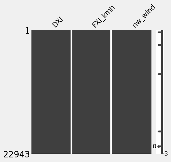
Let’s visualize missing data in the dataset:
ax = msno.matrix(df_cap, figsize=(5, 5))

Wind direction
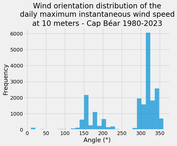
The distribution of wind direction at Cap Béar, specifically the direction of daily maximum instantaneous wind speeds measured at 10 meters, is shown below:
ax = df_cap["DXI"].plot.hist(bins=30, alpha=0.7)
_ = ax.set(
    title="Wind orientation distribution of the\ndaily maximum instantaneous wind speed\nat 10 meters - Cap Béar 1980-2023",
    xlabel="Angle (°)",
)
Number of tramontane days per year
For this analysis, a day is classified as a tramontane day if the wind comes from a north-west direction with gusts exceeding 60 km/h. One limitation is that we don’t account for the timing of the maximum wind speed. We look at the maximum wind speed measured over a 24-hour period from midnight to midnight. If the wind picks up in the evening and stops early the next morning, it would count as two separate days.
We count the number of such days per year and apply linear, quadratic, and cubic regression to observe trends:
def plot_number_of_days(
    series: pd.Series,
    start: str = "1980",
    end: str = "2023",
    place: str = "Cap Béar",
    reg_order: int = 3,
    figsize=(15, 7),
    r=11,
):

    ax = series.loc[start:end].plot(
        marker="o", linestyle="", figsize=figsize, alpha=0.7, label="Number of days"
    )

    # linear regression
    if reg_order > 0:
        X = series.index.year.values[:, np.newaxis]
        scaler = RobustScaler()
        X_s = scaler.fit_transform(X)
        y = series.values
        lr = LinearRegression()
        lr.fit(X_s, y)
        reg = pd.Series(data=lr.predict(X_s), index=series.index)
        ax = reg.plot(
            ax=ax, linewidth=1.5, color="k", label="Linear regression", alpha=0.6
        )

    # quadratic regression
    if reg_order > 1:
        X = series.index.year.values[:, np.newaxis]
        poly = PolynomialFeatures(2)
        X = poly.fit_transform(X)
        scaler = RobustScaler()
        X_s = scaler.fit_transform(X)
        y = series.values
        lr = LinearRegression()
        lr.fit(X_s, y)
        reg = pd.Series(data=lr.predict(X_s), index=series.index)
        ax = reg.plot(
            ax=ax,
            linewidth=1.5,
            linestyle="-.",
            color="k",
            label="Quadratic regression",
            alpha=0.6,
        )

    # cubic regression
    if reg_order > 2:
        X = series.index.year.values[:, np.newaxis]
        poly = PolynomialFeatures(3)
        X = poly.fit_transform(X)
        scaler = RobustScaler()
        X_s = scaler.fit_transform(X)
        y = series.values
        lr = LinearRegression()
        lr.fit(X_s, y)
        reg = pd.Series(data=lr.predict(X_s), index=series.index)
        ax = reg.plot(
            ax=ax,
            linewidth=1.5,
            linestyle=":",
            color="k",
            label="Cubic regression",
            alpha=0.6,
        )

    # rolling window  mean
    ax = (
        series.loc[start:end]
        .rolling(r, center=True)
        .mean()
        .plot(ax=ax, alpha=0.6, label=f"rolling({r}) mean")
    )

    _ = ax.set(
        title=f"Nomber of tramontane days per year - {place}",
        xlabel="Year",
    )
    _ = ax.set_xlim(f"{int(start)-1}", f"{int(end)+1}")
    _ = ax.set_ylim(
        0,
    )
    _ = ax.legend()

    return ax
tramontane_days_cap = (
    df_cap.loc[(df_cap.nw_wind == 1) & (df_cap.FXI_kmh >= 60.0)].resample("YS").size()
)

ax = plot_number_of_days(tramontane_days_cap, place="Cap Béar")
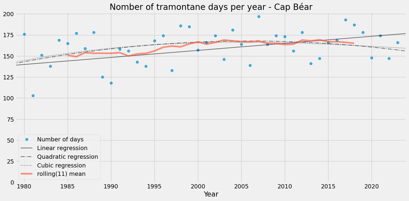
Tramontane frequency appears to have increased, reaching a peak around 2010 to 2015, and may have since declined.
Perpignan (66)

Par Martine SODAIGUI — Travail personnel, CC BY-SA 3.0, https://commons.wikimedia.org/w/index.php?curid=29726806
Loading Data for Perpignan
df_per = df_all[df_all.NOM_USUEL == "PERPIGNAN"].copy(deep=True)
df_per = df_per.dropna(how="all")
df_per = df_per.asfreq("d")
df_per = df_per.drop("NOM_USUEL", axis=1)
df_per.head(3)
| DXI | FXI_kmh | nw_wind | |
|---|---|---|---|
| date | |||
| 1962-01-01 | 40.0 | 32.4 | 0.0 |
| 1962-01-02 | 320.0 | 32.4 | 1.0 |
| 1962-01-03 | 320.0 | 68.4 | 1.0 |
ax = msno.matrix(df_per, figsize=(5, 5))
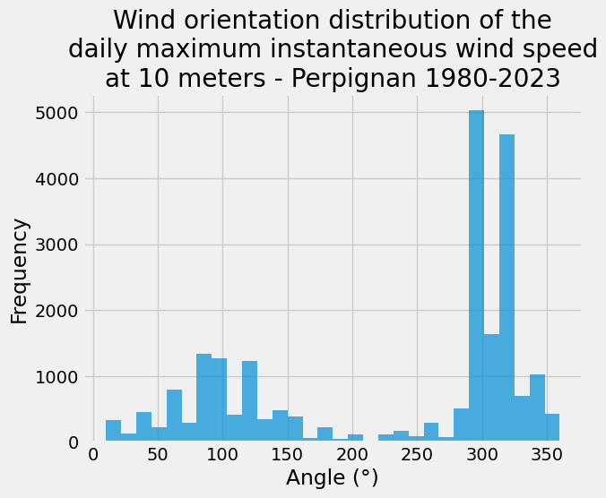
Wind direction
ax = df_per["DXI"].plot.hist(bins=30, alpha=0.7)
_ = ax.set(
    title="Wind orientation distribution of the\ndaily maximum instantaneous wind speed\nat 10 meters - Perpignan 1980-2023",
    xlabel="Angle (°)",
)
Number of tramontane days per year
tramontane_days_per = (
    df_per.loc[(df_per.nw_wind == 1) & (df_per.FXI_kmh >= 60.0)].resample("YS").size()
)

ax = plot_number_of_days(tramontane_days_per, place="Perpignan")
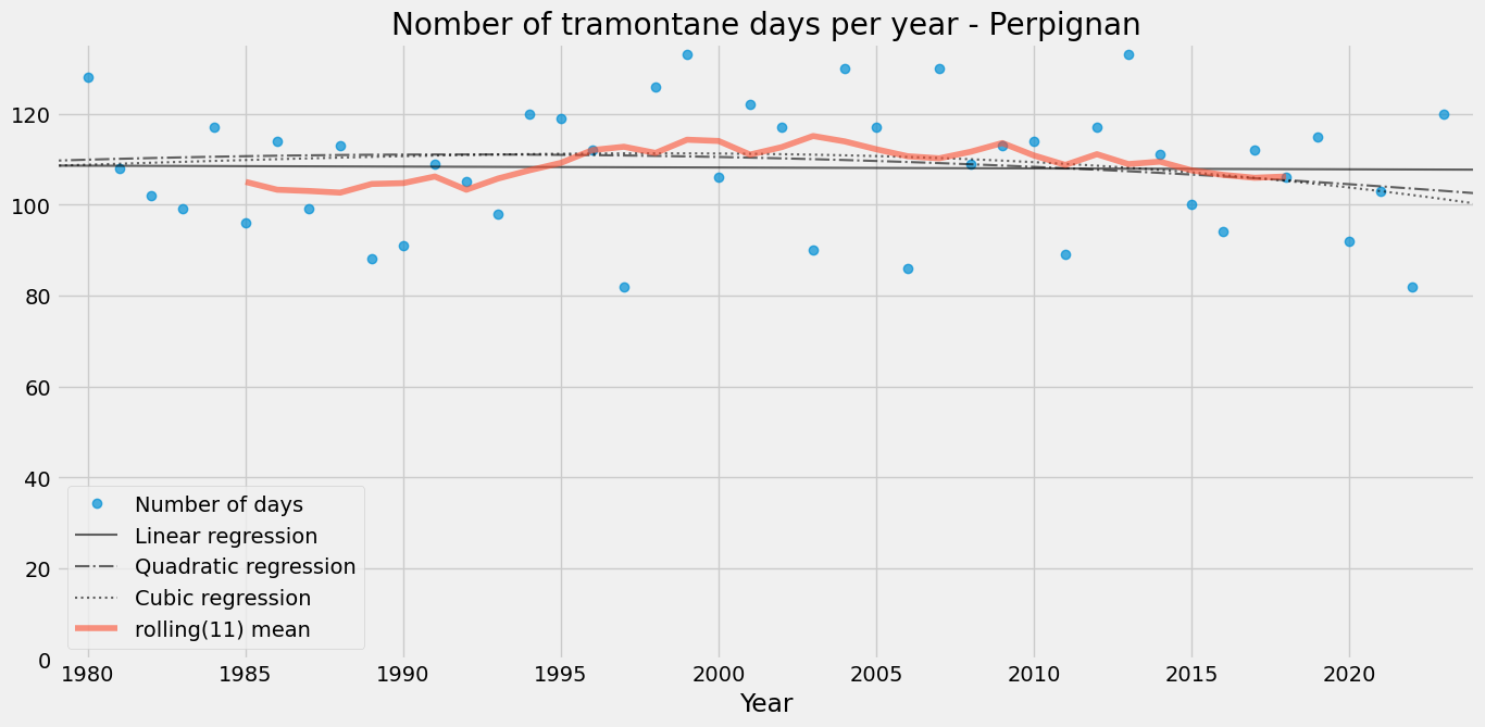
In Perpignan, the tramontane frequency has remained relatively stable.
Leucate (11)

Par BlueBreezeWiki — Travail personnel, CC BY-SA 3.0, https://commons.wikimedia.org/wiki/File:110527-Leucate-01.jpg
Loading Data for Leucate
df_leu = df_all[df_all.NOM_USUEL == "LEUCATE"].copy(deep=True)
df_leu = df_leu.dropna(how="all")
df_leu = df_leu.asfreq("d")
df_leu = df_leu.drop("NOM_USUEL", axis=1)
df_leu.head(3)
| DXI | FXI_kmh | nw_wind | |
|---|---|---|---|
| date | |||
| 1995-03-21 | 310.0 | 68.4 | 1.0 |
| 1995-03-22 | 30.0 | 54.0 | 0.0 |
| 1995-03-23 | 30.0 | 32.4 | 0.0 |
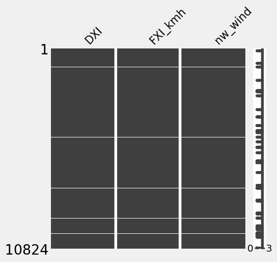
ax = msno.matrix(df_leu, figsize=(5, 5))
Wind direction
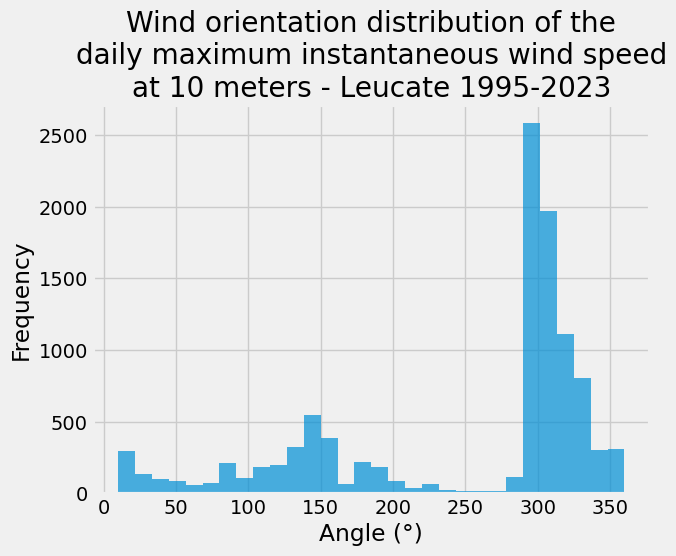
ax = df_leu["DXI"].plot.hist(bins=30, alpha=0.7)
_ = ax.set(
    title="Wind orientation distribution of the\ndaily maximum instantaneous wind speed\nat 10 meters - Leucate 1995-2023",
    xlabel="Angle (°)",
)
Number of tramontane days per year
tramontane_days_leu = (
    df_leu.loc[(df_leu.nw_wind == 1) & (df_leu.FXI_kmh >= 60.0)].resample("YS").size()
)

ax = plot_number_of_days(tramontane_days_leu, place="Leucate", start="1995")
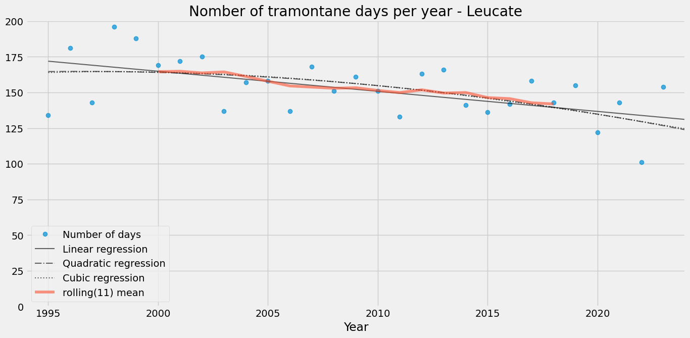
In Leucate, the decreasing trend is evident, with about 30 to 40 fewer tramontane days per year since 1995.
Conclusion
The trends for Cap Béar and Perpignan are not very clear to me at this time, although there appears to be a recent decrease in frequency. In contrast, Leucate shows a clear decreasing trend in tramontane wind days over time.
However, long-term weather models suggest that the tramontane frequency is expected to decline in the future. For more details, see the relevant study by Obermann-Hellhund et al. [1]:
The five simulations with three RCMs [Regional Climate Models] and five GCMs [General Circulation Models] in this study show only small changes in Mistral frequency in RCP4.5 [Representative Concentration Pathways, climate change scenarios] and RCP8.5 projections, but a significant decrease in Tramontane frequency. Most GCMs and RCMs show a decrease in Tramontane days per year, but changes are stronger in RCM simulations. This leads to the conclusion that future climate could lead to a change in Tramontane frequency, while the average wind speed during Tramontane events is not projected to change.
Citation
[1] Obermann-Hellhund, A., Conte, D., Somot, S. et al. Mistral and Tramontane wind systems in climate simulations from 1950 to 2100. Clim Dyn 50, 693–703 (2018).https://doi.org/10.1007/s00382-017-3635-8 pdf
Bonus : the 3, 6, 9 days rule
The inhabitants of the Languedoc-Roussillon region refer to the “rule of 3, 6, 9,” which suggests that when the tramontane wind rises, it may blow for 3, 6, or 9 days. Let’s test this rule in Perpignan.
df_per["tram"] = -1  # no data
df_per.loc[(df_per.nw_wind == 1) & (df_per.FXI_kmh >= 60), "tram"] = 1  # tramontane day
df_per.loc[(df_per.nw_wind == 0) | (df_per.FXI_kmh < 60), "tram"] = 0  # not a tramontane day
df_per.tram.value_counts()
tram
 0    15598
 1     6823
-1      522
Name: count, dtype: int64
Now let’s analyze the number of consecutive tramontane days:
df = df_per[["tram"]].copy(deep=True)

df["group"] = (df["tram"] != df["tram"].shift()).cumsum()  # identify groups of consecutive 1s

# iterate over each group and sum the consecutive 1s
df["summed"] = df["tram"]
for group, group_df in df.groupby("group"):
    if group_df["tram"].iloc[0] == 1:
        summed_value = group_df["tram"].sum()
        df.loc[group_df.index[0], "summed"] = summed_value
        df.loc[group_df.index[1:], "summed"] = 0

df = df.drop(columns=["group"])

counts = df.loc[df.summed > 0, "summed"].value_counts()
counts = counts.sort_index()
new_index = range(counts.index.min(), counts.index.max() + 1)
counts = counts.reindex(new_index, fill_value=0)
s = counts / counts.sum()  # normalize the distribution
ax = s.plot.bar(alpha=0.7, figsize=(15, 7), rot=45)

_ = ax.set(
    title="Distribution of the number of consecutive tramontane days in Perpignan 1980-2023",
    xlabel="Number of consectutive tramontane days",
    ylabel="Propability",
)
_ = ax.set_xlim(-1, 14)
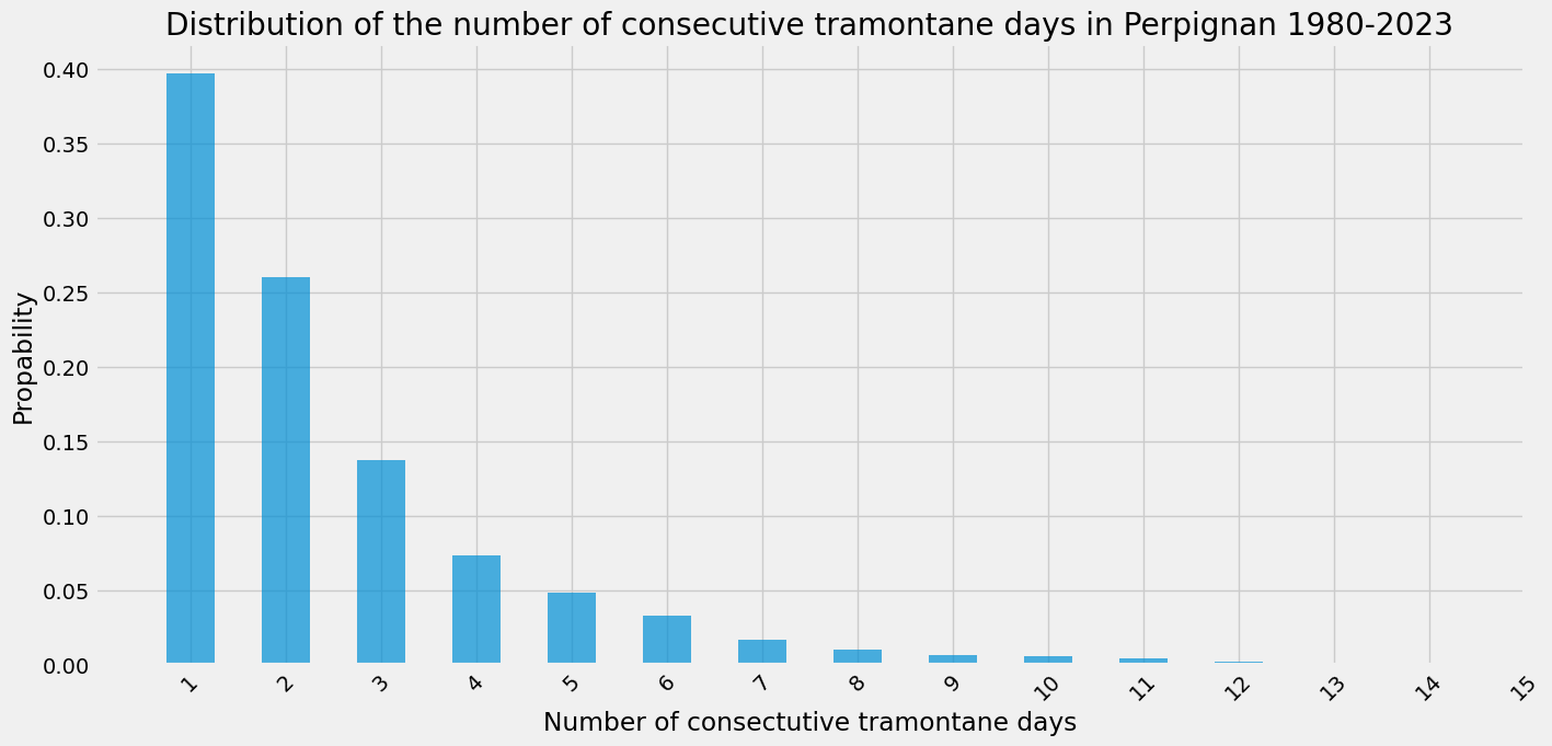
Let’s fit a discrete exponential distribution to this data:
\[P(X=k) = \beta \; e^{-\alpha \; k}, \; k \geq 1\]To normalize the distribution, we use the following identity:
\[\sum_{k=1}^{\infty} P(X=k) = \frac{\beta}{e^{\alpha}-1} = 1\]This results in a simplified formula:
\[P(X=k) = (e^{\alpha}-1) e^{-\alpha \; k}, \; k \geq 1\]def exponential_func(x, alpha):
beta = np.exp(alpha) - 1.0
return beta * np.exp(-alpha * x)
x_data = np.array(s.index)
y_data = s.values
alpha_0 = 0.1
popt, pcov = curve_fit(exponential_func, x_data, y_data, p0=alpha_0)
# Extract the parameters
alpha = popt[0]
beta = np.exp(alpha) - 1.0
print(f"Fitted parameter: alpha = {alpha}")
Fitted parameter: alpha = 0.5182052615562184
exp = pd.Series(index=x_data, data=exponential_func(x_data, alpha))
exp.name = "Fitted exponential distribution"
s.name = "Observed"
ax = s.plot(alpha=0.3, marker='o', ms=20, figsize=(15, 7), rot=45)
ax = exp.plot(ax=ax, alpha=0.8)
_ = ax.set(
    title="Fitted distribution of the number of consecutive tramontane days\n in Perpignan 1980-2023",
    xlabel="Number of consectutive tramontane days",
    ylabel="Propability",
)
_ = ax.set_xlim(0, 15)
_ = ax.legend()
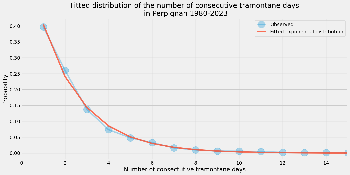
The distribution of consecutive tramontane days in Perpignan is rather well approximated by an exponential distribution, as shown by the fitted curve. It seems to follow a continuous and predictable pattern, without any noticeable anomalies such as the 3, 6, 9-day rule.