In-memory cosine distance calculation, NumPy vs DuckDB
This notebook compares the performance of NumPy and DuckDB for computing cosine distances on the same dataset.
The dataset is dbpedia_14 with 630,073 embedded text chunks of wikipedia text. The embedding model is distilbert-dot-tas_b-b256-msmarco with an embedding dimension of 768. Check this post to see how the embedding vectors were created: A Hybrid information retriever with DuckDB.
The data is located on the disk as a .duckdb database file. We are going to load the data as an in-memory DuckDB database and a NumPy array as well.
Outline
Imports and package versions
import duckdb
import numpy as np
import pandas as pd
Package versions:
Python               : 3.13.0
duckdb               : 1.2.0
numpy                : 2.2.3
pandas               : 2.2.3
Query with DuckDB
Load the data into memory
We load the dataset from disk into an in-memory DuckDB database to enable fast queries and computations.
con = duckdb.connect()
query = "ATTACH '/home/francois/Workspace/Search_PDFs/dbpedia_14.duckdb' AS disk;"
con.sql(query)
%%time
query = """
CREATE TABLE dbpedia_14 AS (
  SELECT chunk_index, title, chunk_embedding
  FROM disk.dbpedia_14
  ORDER BY chunk_index);"""
con.sql(query)
CPU times: user 9.17 s, sys: 2.59 s, total: 11.8 s
Wall time: 3.66 s
query = "SELECT COUNT(*) FROM dbpedia_14"
con.sql(query)
┌──────────────┐
│ count_star() │
│    int64     │
├──────────────┤
│       630073 │
└──────────────┘
So we have 630073 vectors of size 768:
query = """
SELECT data_type
FROM information_schema.columns
WHERE table_catalog = 'memory'
  AND table_name = 'dbpedia_14'
  AND column_name = 'chunk_embedding';"""
con.sql(query)
┌────────────┐
│ data_type  │
│  varchar   │
├────────────┤
│ FLOAT[768] │
└────────────┘
Normalize the embedding vectors in-place
We first normalize the embedding vectors by dividing them by their L2 norm. While this process is computationally expensive, it is performed only once and eliminates redundant calculations during later similarity searches.
Checking the L2 norm confirms that the vectors are unnormalized, with the first vector of the column:
query = "SELECT chunk_embedding FROM dbpedia_14 LIMIT 1"
search_embedding = con.sql(query).fetchnumpy()["chunk_embedding"][0]
np.linalg.norm(search_embedding, 2)
np.float32(11.047098)
The normalization is done here as a two-step process. First, we compute the L2 norm of each vector and store it in the l2_norm column:
%%time
query = """
ALTER TABLE dbpedia_14 ADD COLUMN IF NOT EXISTS l2_norm FLOAT;
UPDATE dbpedia_14
SET l2_norm = sqrt(list_sum(list_transform(chunk_embedding, y -> y * y)));"""
con.sql(query)
CPU times: user 3.32 s, sys: 557 ms, total: 3.87 s
Wall time: 765 ms
Now, we divide each embedding by its precomputed norm:
%%time
query = """
UPDATE dbpedia_14
SET chunk_embedding = list_transform(chunk_embedding, x -> x / l2_norm);"""
con.sql(query)
CPU times: user 4.04 s, sys: 385 ms, total: 4.43 s
Wall time: 2.44 s
Select the element to search against
To perform a similarity search, we first select an element from the dataset so that we can find the 5 most similar vectors in the table, i.e. with the smallest cosine distance value. We retrieve the entry with chunk_index = 0:
query = "SELECT chunk_index, title FROM dbpedia_14 WHERE chunk_index = 0"
con.sql(query)
┌─────────────┬──────────────────┐
│ chunk_index │      title       │
│    int64    │     varchar      │
├─────────────┼──────────────────┤
│           0 │ E. D. Abbott Ltd │
└─────────────┴──────────────────┘
Next, we extract its corresponding embedding:
query = "SELECT chunk_embedding FROM dbpedia_14 WHERE chunk_index = 0"
search_embedding = con.sql(query).fetchnumpy()["chunk_embedding"][0]
To confirm that our normalization step was successful, we check that the L2 norm of this embedding is 1:
np.linalg.norm(search_embedding, 2)
np.float32(1.0)
Cosine distance query
The cosine distance $D(u,v)$ between two vectors $u$ and $v$ is defined as:
\[D(u, v) = 1- \frac{u \cdot v}{\|u\|_2 \|v\|_2}\]This is not strictly a “distance” in the mathematical sense, as it does not satisfy the triangle inequality. Since we have normalized our embeddings, their L2 norms are 1, simplifying the equation to:
\[D(u, v) = 1 - u \cdot v\]Thus, computing the cosine distance reduces to computing the dot/inner product. We are going to use the array_negative_inner_product function to compute $(- u \cdot v)$.
%%timeit -r 10 -n 1
query = f"""
SELECT chunk_index, title, 1 + array_negative_inner_product(
  chunk_embedding,
  Cast(? AS FLOAT[768]))
  AS cosine_distance
FROM dbpedia_14
ORDER BY cosine_distance ASC
LIMIT 5;"""
con.execute(query, (search_embedding,)).df()
165 ms ± 6.46 ms per loop (mean ± std. dev. of 10 runs, 1 loop each)
| chunk_index | title | cosine_distance | |
|---|---|---|---|
| 0 | 0 | E. D. Abbott Ltd | 0.000000 |
| 1 | 219729 | Abbott Farnham sailplane | 0.112158 |
| 2 | 31145 | Abbott-Baynes Sailplanes | 0.139073 |
| 3 | 38684 | Abbott-Detroit | 0.142139 |
| 4 | 34947 | East Lancashire Coachbuilders | 0.153380 |
Query with NumPy
Load the data into NumPy
To perform similarity searches with NumPy, we first load all embeddings from the .duckdb file into a NumPy array.
%%time
sql = "SELECT chunk_embedding FROM disk.dbpedia_14 ORDER BY chunk_index"
embeddings = con.execute(sql).fetchnumpy()["chunk_embedding"]
embeddings = np.vstack(embeddings)
CPU times: user 5.14 s, sys: 1.65 s, total: 6.79 s
Wall time: 3.52 s
After loading, we verify the shape of the array:
embeddings.shape
(630073, 768)
To confirm that the embeddings are not yet normalized, we check the L2 norm of the first vector:
np.linalg.norm(embeddings[0, :], 2)
np.float32(11.047098)
Normalize the embedding vectors
Note that we could have used the normalized vectors from DuckDB that are already in memory. We instead started independently from the data on disk and normalize the NumPy way:
%%time
norms = np.linalg.norm(embeddings, ord=2, axis=1)
embeddings /= norms[:, np.newaxis]
CPU times: user 451 ms, sys: 2.64 s, total: 3.09 s
Wall time: 3.18 s
np.linalg.norm(embeddings[0, :], 2)
np.float32(0.99999994)
Select the element to search against
We use the same reference element as before, now extracted from the NumPy array of normalized embeddings:
search_embedding = embeddings[0]
Cosine distance query
We calculate the cosine distance using the formula $D(u,v)=1− u \cdot v$:
cosine_distances = 1.0 - np.dot(embeddings, search_embedding)
To efficiently retrieve the top 5 closest results, we use np.argpartition to find the indices of the smallest cosine distances, and then sort those indices to get the final results:
%%timeit -r 10 -n 1
cosine_distances = 1.0 - np.dot(embeddings, search_embedding)
k = 5
smallest_indices = np.argpartition(cosine_distances, k)[:k]
smallest_indices = smallest_indices[np.argsort(cosine_distances[smallest_indices])]
smallest_values = cosine_distances[smallest_indices]
pd.DataFrame({"chunk_index": smallest_indices, "cosine_distance": smallest_values})
36.1 ms ± 2.86 ms per loop (mean ± std. dev. of 10 runs, 1 loop each)
| chunk_index | cosine_distance | |
|---|---|---|
| 0 | 0 | 0.000000 |
| 1 | 219729 | 0.112157 |
| 2 | 31145 | 0.139073 |
| 3 | 38684 | 0.142139 |
| 4 | 34947 | 0.153380 |
The top 5 closest elements are the same chunk indexes as those found earlier with DuckDB, with same distance. We can directly compare the chunk index from the database table with the NumPy array index because the embeddings were loaded using ORDER BY chunk_index, and it contains contiguous integers starting at 0.
Finally, we ensure that the database is properly detached from DuckDB, and the connection is closed.
query = "DETACH disk;"
con.sql(query)
con.close()
Results
We compared the elapsed times for computing the cosine distance using both DuckDB and NumPy on the same in-memory data. As shown in the bar chart below, NumPy performs the computation faster than DuckDB.
timings = pd.Series({"DuckDB": 165, "NumPy": 36.1}).to_frame("elapsed_time_ms")
ax = timings.plot.bar(alpha=0.7, grid=True, legend=False, rot=45)
_ = ax.set(title="Comparing cosine distance computation in-memory:\nDuckDB vs NumPy on the dbpedia_14 Dataset", ylabel="Elapsed time (ms)")
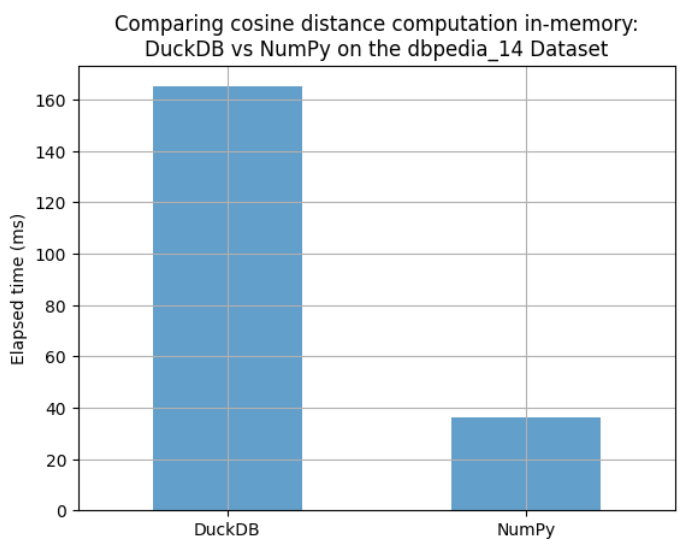
However, these are two different tools with very distinct purposes. NumPy is based on highly optimized linear algebra libraries, which likely explains the observed performance difference in this small brute-force search example. But of course, for any real-world vector search application, a database with vector support is essential: disk-based storage with persistence, advanced indexing techniques, memory mapping to handle large datasets efficiently, while enabling concurrent queries and filtering, and so on… This post is only meant for benchmarking computational time.