Spatial queries in DuckDB with R-tree and H3 indexing
This Python notebook explores the use of two indexing techniques, R-tree and H3, for performing spatial queries in DuckDB. The motivation behind this is to analyze a dataset of 31 million rows containing geographical coordinates, and to efficiently select all rows within a 1 km radius of a given point.
Imports and package versions
import contextily as cx
import datashader as ds
import duckdb
import geopandas as gpd
import h3
import matplotlib.pyplot as plt
import numpy as np
import pandas as pd
import xyzservices.providers as xyz
from colorcet import palette
from datashader import transfer_functions as tf
from pyproj import Transformer
from shapely.geometry import Point, Polygon

DUCK_DB_FP = "./dvf_points.duckdb"  # file path
Versions:
Python               : 3.13.0
contextily           : 1.6.2
datashader           : 0.17.0
duckdb               : 1.2.0
geopandas            : 1.0.1
h3                   : 4.2.1
matplotlib           : 3.10.1
numpy                : 2.1.3
pandas               : 2.2.3
xyzservices          : 2025.1.0
colorcet             : 3.1.0
pyproj               : 3.7.1
shapely              : 2.0.7
The Point dataset
Let’s first explore our dataset. It was extracted from the French “Demandes de Valeurs Foncières” (DVF) with geolocation, a public dataset of real estate transactions across mainland France, excluding Alsace and Moselle. Each row represents a real estate transaction, and our focus in this post will be on the geographical coordinates associated with these transactions.
It is stored in a DuckDB file on disk, and we start by connecting to it:
con = duckdb.connect(DUCK_DB_FP)
The present dataset contains three columns: id, longitude, and latitude. Here’s a quick preview:
query = "SELECT * FROM dvf LIMIT 3"
con.sql(query)
┌───────┬───────────┬───────────┐
│  id   │ longitude │ latitude  │
│ int64 │  double   │  double   │
├───────┼───────────┼───────────┤
│     0 │   4.92463 │ 46.134719 │
│     1 │  4.923909 │ 46.132876 │
│     2 │  4.957296 │ 46.152664 │
└───────┴───────────┴───────────┘
We check for missing values in these columns:
%%time
query = """
SELECT
  COUNT(*) AS total_rows,
  COUNT(*) - COUNT(id) AS missing_id,
  COUNT(*) - COUNT(latitude) AS missing_latitude,
  COUNT(*) - COUNT(longitude) AS missing_longitude
FROM dvf;"""
con.sql(query).show()
┌────────────┬────────────┬──────────────────┬───────────────────┐
│ total_rows │ missing_id │ missing_latitude │ missing_longitude │
│   int64    │   int64    │      int64       │       int64       │
├────────────┼────────────┼──────────────────┼───────────────────┤
│   31030270 │          0 │                0 │                 0 │
└────────────┴────────────┴──────────────────┴───────────────────┘

CPU times: user 376 ms, sys: 177 ms, total: 553 ms
Wall time: 40 ms
We have over 31 million records and no missing values. While each row in our dataset represents a real estate transaction, the geographical coordinates are not necessarily unique. Some transactions share the same latitude and longitude, which we can verify by counting the number of distinct coordinate pairs:
%%time
query = """
SELECT COUNT(*)
FROM (
  SELECT DISTINCT longitude, latitude
  FROM dvf
) AS distinct_pairs;"""
con.sql(query)
CPU times: user 1.86 ms, sys: 183 μs, total: 2.05 ms
Wall time: 1.43 ms


┌──────────────┐
│ count_star() │
│    int64     │
├──────────────┤
│     15986516 │
└──────────────┘
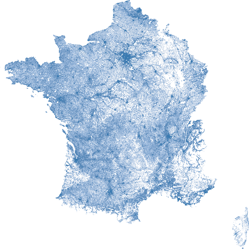
To see the spatial distribution of these points, we can visualize them with datashader:
%%time
cmap = palette["blues"]
bg_col = "white"
size_x, size_y = 1024, 1024
cvs = ds.Canvas(plot_width=size_x, plot_height=size_y)
df = con.execute("SELECT longitude, latitude FROM dvf").df()
agg = cvs.points(df, "longitude", "latitude")
img = tf.shade(agg, cmap=cmap)
img = tf.set_background(img, bg_col)
del df
img
CPU times: user 1.67 s, sys: 212 ms, total: 1.88 s
Wall time: 1.83 s
Creating the Geometry Column
To perform spatial queries efficiently, we need to create a geometry column in our dataset. We start by installing and loading the spatial extension, then add a new column geom to store the geometry representation of each transaction’s coordinates. Finally, we transform the coordinates from EPSG:4326 (WGS 84) to EPSG:2154 (RGF93 / Lambert-93).
The key advantage of using EPSG:2154 is that it is a projected Coordinate Reference System (CRS). This makes it useful for spatial queries involving distance calculations, such as defining a buffer radius around a point. A little surprising detail to me is that when using ST_Point(), the latitude must come first to obtain valid coordinates.
%%time
query = """
INSTALL spatial; LOAD spatial;
ALTER TABLE dvf ADD COLUMN geom GEOMETRY;
UPDATE dvf SET geom = ST_Transform(
  ST_Point(latitude, longitude), 'EPSG:4326', 'EPSG:2154'
);"""
con.sql(query)
CPU times: user 2min 41s, sys: 1min 13s, total: 3min 55s
Wall time: 1min 43s
This takes a while, but only needs to be done once.
Query without index
Let’s first run a spatial query without an index. We will search for all transactions within a 1 km radius around a specific point in Lyon, that we will keep using in the following:
lat, lon = 45.774894216486274, 4.832142311498748
buffer_radius = 1000
Since our geometry column is stored in EPSG:2154 (Lambert-93), we must transform our query point from EPSG:4326 (WGS 84) to match:
transformer = Transformer.from_crs("EPSG:4326", "EPSG:2154", always_xy=True)
x_2154, y_2154 = transformer.transform(lon, lat)
The argument always_xy=True ensures that we enter the longitude first.
Now, let’s run a spatial distance query using ST_DWithin, which selects all transactions within the 1 km buffer:
%%timeit -r 10 -n 1
query = f"""
SELECT id, longitude, latitude FROM dvf
WHERE ST_DWithin(geom, ST_Point({x_2154}, {y_2154}), {buffer_radius});"""
df_select = con.sql(query).df()
1.38 s ± 10.3 ms per loop (mean ± std. dev. of 10 runs, 1 loop each)
At 1.38 seconds per query, this approach is not optimal. The database actually scans all records to find matching points.
df_select.shape
(20831, 3)
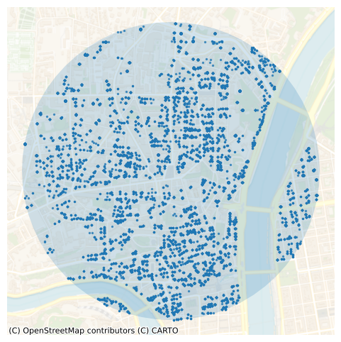
The query returns 20,831 points. Let’s plot the selected transactions along with the 1 km buffer around the target location:
gdf_select_1 = gpd.GeoDataFrame(
    df_select["id"],
    geometry=gpd.points_from_xy(df_select.longitude, df_select.latitude),
    crs="EPSG:4326",
)
gdf_select_1 = gdf_select_1.to_crs("EPSG:2154")
ax = gdf_select_1.plot(markersize=2, alpha=0.7, figsize=(6, 6))
point = Point(x_2154, y_2154)
buffer = point.buffer(buffer_radius)
buffer_gdf = gpd.GeoDataFrame(geometry=[buffer], crs="EPSG:2154")
ax = buffer_gdf.plot(ax=ax, alpha=0.2)
cx.add_basemap(
    ax,
    source=xyz.CartoDB.VoyagerNoLabels,
    crs=gdf_select_1.crs.to_string(),
    alpha=0.8,
)
_ = plt.axis("off")
With an R-tree index
Now let’s see how an R-tree index can improve query performance. First, we create the spatial index on the geom column:
%%time
query = "CREATE INDEX spatial_index ON dvf USING RTREE (geom);"
con.sql(query)
CPU times: user 22.1 s, sys: 304 ms, total: 22.4 s
Wall time: 4.37 s
Let’s test the performance again by running a spatial distance query using ST_DWithin:
%%timeit -r 10 -n 1
query = f"""
SELECT id, longitude, latitude FROM dvf
WHERE ST_DWithin(geom, ST_Point({x_2154}, {y_2154}), {buffer_radius});"""
df_select = con.sql(query).df()
1.39 s ± 17.1 ms per loop (mean ± std. dev. of 10 runs, 1 loop each)
The spatial index is not used with ST_DWithin.
Here is what the Spatial extension’s documentation says:
The R-tree index will only be used to perform “index scans” when the table is filtered (using a
WHEREclause) with one of the following spatial predicate functions (as they all imply intersection):ST_Equals,ST_Intersects,ST_Touches,ST_Crosses,ST_Within,ST_Contains,ST_Overlaps,ST_Covers,ST_CoveredBy,ST_ContainsProperly.
We switch to using ST_Intersects along with ST_Buffer:
%%timeit -r 10 -n 1
query = f"""
SELECT id, longitude, latitude FROM dvf
WHERE ST_Intersects(geom, ST_Buffer(ST_Point({x_2154}, {y_2154}), {buffer_radius}));"""
df_select = con.sql(query).df()
65.3 ms ± 1.22 ms per loop (mean ± std. dev. of 10 runs, 1 loop each)
Now the R-tree index is scanned by the SQL engine, the execution time improves significantly. Note that we might improve the performance with the min_node_capacity and max_node_capacity parameters during the index creation step.
However, this query returns 20,685 points, which is less than before with ST_DWithin (20831):
df_select.shape
(20685, 3)
This is because in the latter case, a polygon with radius 1 km is created first, and some points at the border fall outside the polyogn while being with a 1 km distance from the query point:
-
ST_Intersectswill only include points that touch or fall inside the buffer polygon boundary. -
ST_DWithinwill include all points within the radius.
Let’s visualize these points falling outside.
gdf_select_2 = gpd.GeoDataFrame(
    df_select["id"],
    geometry=gpd.points_from_xy(df_select.longitude, df_select.latitude),
    crs="EPSG:4326",
)
gdf_select_2 = gdf_select_2.to_crs("EPSG:2154")
We merge the results from both ST_DWithin and ST_Intersects to see how the two approaches compare:
merged_gdf = pd.merge(
    gdf_select_1[["id", "geometry"]],
    gdf_select_2[["id"]],
    on="id",
    how="outer",
    indicator=True,
)
merged_gdf._merge.value_counts()
_merge
both          20685
left_only       146
right_only        0
Name: count, dtype: int64
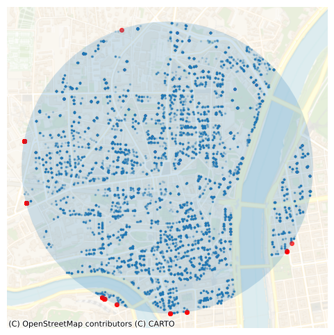
The query with ST_Intersects excludes 146 points (in red) that were included in the ST_DWithin query.
ax = merged_gdf.loc[merged_gdf._merge == "both", "geometry"].plot(
    markersize=2, alpha=0.2, figsize=(6, 6)
)
ax = merged_gdf.loc[merged_gdf._merge == "left_only", "geometry"].plot(
    markersize=16, color="r", alpha=0.7, ax=ax
)
point = Point(x_2154, y_2154)
buffer = point.buffer(buffer_radius)
buffer_gdf = gpd.GeoDataFrame(geometry=[buffer], crs="EPSG:2154")
ax = buffer_gdf.plot(ax=ax, alpha=0.2)
cx.add_basemap(
    ax,
    source=xyz.CartoDB.VoyagerNoLabels,
    crs=buffer_gdf.crs.to_string(),
    alpha=0.8,
)
_ = plt.axis("off")
Note that without any index, both queries, ST_DWithin and ST_Intersects, takes the same amount of time (around 1.38s).
With an H3 index
Now, let’s explore the H3 index. First, we install and load the h3 extension into DuckDB:
query = """
INSTALL h3 FROM community; LOAD h3;"""
con.sql(query)
We drop the previous R-tree index to only take the H3 index into account.
query = """
DROP INDEX IF EXISTS spatial_index;"""
con.sql(query)
The H3 indexing system allows us to represent geographic areas as cells on a hexagonal grid. These cells have different resolutions, which affect the size of the areas they cover. For resolution 7, the average edge length is approximately 1.4 km, as listed in the H3’s documuntation.
We want to select the H3 cell containing our query point, then its first-ring neighbors, retrieve all points within these cells, and finally run ST_Intersects with a buffer around the query point on these selected points. Let’s visualize the buffer, the hexagonal cell and its first-ring neighbors with a resolution of 7. In order to do that, we use the Python h3-py library.
RESOLUTION = 7
# Get H3 cell and neighbors
h3_cell = h3.latlng_to_cell(lat, lon, RESOLUTION)
h3_neighbors = h3.grid_disk(h3_cell, 1)  # Center + 1st ring


# Convert to GeoDataFrame
def h3_to_polygon(h3_index):
    boundary = h3.cell_to_boundary(h3_index)  # Returns [(lat, lon), ...]
    boundary_lonlat = [
        (lon, lat) for lat, lon in boundary
    ]  # Swap to (lon, lat) for Shapely
    return Polygon(boundary_lonlat)


h3_gdf = gpd.GeoDataFrame(
    {"h3": list(h3_neighbors)},
    geometry=[h3_to_polygon(h) for h in h3_neighbors],
    crs="EPSG:4326",
)
h3_gdf = h3_gdf.to_crs("EPSG:2154")
ax = h3_gdf.boundary.plot(color="blue",  alpha=0.7, figsize=(8, 8))
ax = h3_gdf[h3_gdf["h3"] == h3_cell].boundary.plot(ax=ax, color="red", alpha=0.7, linewidth=2)
_ = plt.scatter(
    x_2154, y_2154, color="k", marker="*", label="Input Point"
)
ax = buffer_gdf.plot(ax=ax, alpha=0.4)
cx.add_basemap(
    ax,
    source=xyz.CartoDB.VoyagerNoLabels,
    crs=h3_gdf.crs.to_string(),
    alpha=0.8,
)
_ = plt.axis("off")
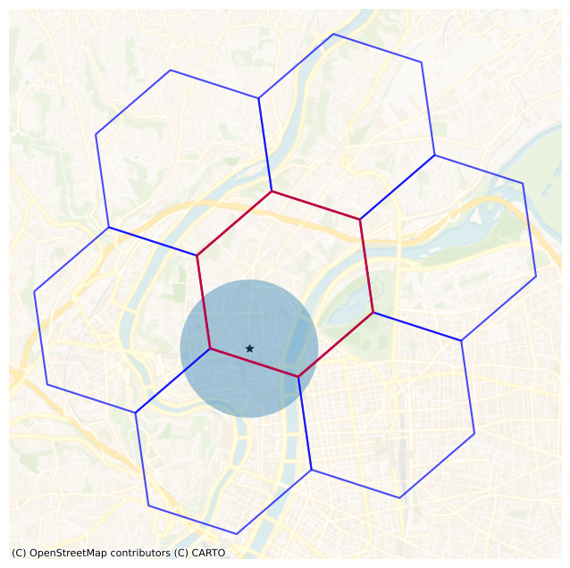
Well the resolution is fine. We do not want to cover too much area with the 1st ring of cells, but we also need to make sure that the buffer is fully included. With a resolution of 8, the edge length is around 531 m, which might be enough. But let’s take a safety margin. Note that we could also add the 2nd ring neighbors with resolution 8.
Let’s add an h3_cell_id column to our dataset and create an index on it for faster querying:
%%time
query = f"""
ALTER TABLE dvf ADD COLUMN IF NOT EXISTS h3_cell_id BIGINT;
UPDATE dvf
  SET h3_cell_id = h3_latlng_to_cell(latitude, longitude, {RESOLUTION});
CREATE INDEX h3_index ON dvf (h3_cell_id)"""
con.sql(query)
CPU times: user 39.4 s, sys: 2.94 s, total: 42.3 s
Wall time: 4.35 s
Finally, let’s run a query using the h3 index. We will use the h3_latlng_to_cell function to select the H3 cell corresponding to our point, and h3_grid_disk to get its neighboring cells:
%%timeit -r 10 -n 1
query = f"""
WITH query_h3 AS (
  SELECT h3_latlng_to_cell({lat}, {lon}, {RESOLUTION}) AS h3
),
nearby_h3 AS (
  SELECT CAST(unnest(h3_grid_disk(h3, 1)) AS BIGINT) AS h3 FROM query_h3
)
SELECT dvf.*
FROM dvf
INNER JOIN nearby_h3 ON dvf.h3_cell_id = nearby_h3.h3
WHERE ST_Intersects(geom, ST_Buffer(ST_Point({x_2154}, {y_2154}), {buffer_radius}));"""
df_select = con.sql(query).df()
28.4 ms ± 2.6 ms per loop (mean ± std. dev. of 10 runs, 1 loop each)
This is an improvement in query performance.
df_select.shape
(20685, 5)
con.close()
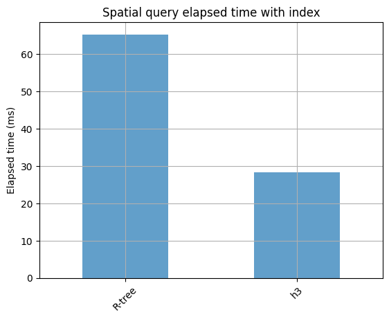
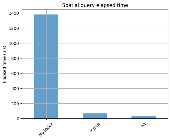
Results
timings = pd.Series({"No index": 1380, "R-tree": 65.3, "h3": 28.4}).to_frame(
    "elapsed_time_ms"
)
ax = timings.plot.bar(alpha=0.7, grid=True, legend=False, rot=45)
_ = ax.set(title="Spatial query elapsed time", ylabel="Elapsed time (ms)")
ax = timings.iloc[1:].plot.bar(alpha=0.7, grid=True, legend=False, rot=45)
_ = ax.set(title="Spatial query elapsed time with index", ylabel="Elapsed time (ms)")