Arnold tongues with Numba, Numba CUDA and Datashader
This Python notebook explores Arnold tongues. Here is a short description from wikipedia:
In mathematics, particularly in dynamical systems, Arnold tongues (named after Vladimir Arnold) are a pictorial phenomenon that occur when visualizing how the rotation number of a dynamical system, or other related invariant property thereof, changes according to two or more of its parameters. The regions of constant rotation number have been observed, for some dynamical systems, to form geometric shapes that resemble tongues, in which case they are called Arnold tongues.
In simpler terms, Arnold tongues represent regions where two oscillating systems synchronize in interesting ways. So an oscillator with its natural frequency may be forced by another oscillator at a different frequency, depending on the forcing parameters. On a parameter plot:
- The horizontal axis represents the frequency of the forcing oscillator
- The vertical axis represents the amplitude (strength) of the forcing
Within the tongue-shaped regions, the original oscillator synchronizes with the forcing oscillator, either matching its frequency exactly or locking onto a rational multiple of it. This phenomenon is known as frequency locking or mode locking. These rational frequency ratio $p/q$ are such that the integers $p$ and $q$ are relative primes.
These tongues are named after Vladimir Arnold, a great Russian mathematician known for his contributions to many fields.

Vladimir Arnold. Source: Wikimedia Commons. This file is licensed under the Creative Commons Attribution 4.0 International license.
We will focus on the computational efficiency of calculating these regions using Numba on the CPU and on the GPU. Additionally, we will visualize some phase diagrams using Datashader.
This type of computation is ideal for parallelization since the parameter space is two-dimensional and can be easily partitioned into smaller rectangular regions. Most importantly, each grid point calculation is completely independent of the others, making it a perfect candidate for massive parallelism without any synchronization overhead.
Outline
- Imports and package versions
- The Circle Map
- CPU Implementation
- GPU Implementation
- GPU Performance Speedup
- High-Resolution Arnold Tongues with CUDA
Imports and package versions
from time import perf_counter

import datashader as ds
import datashader.transfer_functions as tf
import matplotlib.pyplot as plt
import numpy as np
import pandas as pd
from colorcet import palette
from numba import cuda, jit, prange
package versions:
Python implementation: CPython
Python version       : 3.13.2

datashader: 0.17.0
matplotlib: 3.10.1
numpy     : 2.1.3
pandas    : 2.2.3
numba     : 0.61.0
colorcet  : 3.1.0
The Circle Map
We’ll use a standard sine map, for $n \geq 0$:
\[\theta_{n+1}=\theta_n + \Omega + \hat{K} \sin(2 \pi \theta_n)\]where:
- $\theta$ is the phase
- $\Omega \in [0, 1]$ is the frequency ratio
- $\hat{K}\in[0,1]$ is directly related to the coupling strength $K$, as $\hat{K} = \frac{K}{2 \pi}$
$\Omega$ and $\hat{K}$ are fixed parameters. We start with $\theta_0 = 0$.
Because we are dealing with a circle map, $\theta_{n}$ is computed modulo 1. This ensures:
\[0 \leq \theta_n < 1\]We compute the rotation number $\omega$, or also called the winding number, which is defined as:
\[\omega = \lim_{n \to\infty} \frac{\theta_n-\theta_0}{n}\]This rotation number represents the average increase in phase per iteration, characterizing the long-term behavior of the system.
In all the following we plot rotation numbers for $0 \leq \Omega \leq 1$ and $0 \leq \hat{K} \leq 1/2$.
CPU Implementation
First parallel implementation
First, let’s implement our circle map function with Numba acceleration. The @jit decorator compiles this function to machine code for faster execution:
@jit(nopython=True, fastmath=True)
def circle_map_cpu(theta, omega, k):
    """
    Single iteration of the circle map.

    Args:
        theta: Current phase
        omega: Frequency ratio parameter
        k: Coupling strength parameter

    Returns:
        New phase (modulo 1)
    """
    return (theta + omega + k * np.sin(2.0 * np.pi * theta)) % 1.0
Next, we compute the rotation number:
@jit(nopython=True, fastmath=True)
def compute_rotation_number_cpu(omega, k, num_iter, transient=1_000):
    """
    Compute the rotation number for given parameters.

    Args:
        omega: Frequency ratio parameter
        k: Coupling strength parameter
        num_iter: Number of iterations for averaging
        transient: Number of initial iterations to discard

    Returns:
        Computed rotation number
    """
    # Discard transient behavior
    theta = 0.0
    for i in range(transient):
        theta = circle_map_cpu(theta, omega, k)

    # Remember position after transient
    initial_theta = theta

    # Compute for specified iterations
    for i in range(num_iter):
        theta = circle_map_cpu(theta, omega, k)

    # Calculate rotation number
    total_rot = (theta - initial_theta) % 1.0
    return total_rot / num_iter
Now we’ll compute rotation numbers across a grid of parameter values, using Numba’s parallel execution capabilities with prange:
@jit(nopython=True, parallel=True, fastmath=True)
def compute_all_cpu(n_omega=1000, n_k=500, num_iter=10_000):
    """
    Compute rotation numbers for a grid of parameters.

    Args:
        n_omega: Number of points along the omega axis
        n_k: Number of points along the k axis
        num_iter: Number of iterations for each computation

    Returns:
        k_values: Array of k values
        omega_values: Array of omega values
        rotation_numbers: 2D array of rotation numbers
    """
    # Create parameter grids
    omega_values = np.linspace(0.0, 1.0, n_omega)
    k_values = np.linspace(0.0, 0.5, n_k)
    rotation_numbers = np.zeros((n_k, n_omega))

    # Compute rotation number for each parameter pair
    for i in prange(n_k):
        for j in range(n_omega):
            rotation_numbers[i, j] = compute_rotation_number_cpu(
                omega_values[j], k_values[i], num_iter
            )

    return k_values, omega_values, rotation_numbers
Let’s run the computation with a small parameter grid:
%%time
k_values, omega_values, rotation_numbers = compute_all_cpu(
    n_omega=2000, n_k=1000, num_iter=10_000
)
CPU times: user 16min 55s, sys: 240 ms, total: 16min 55s
Wall time: 1min 7s
The discrepancy between user time and wall time demonstrates Numba’s parallel execution efficiency. The CPU is an Intel i9-12900H with 20 cores. Next, we’ll prepare the data for visualization:
def create_dataframe(k_values, omega_values, rotation_numbers):
    """
    Create a DataFrame from the rotation_numbers.

    Args:
        k_values: Array of k values
        omega_values: Array of omega values
        rotation_numbers: 2D array of rotation numbers

    Returns:
        DataFrame in long format suitable for visualization
    """
    df = pd.DataFrame(rotation_numbers, columns=omega_values, index=k_values)
    df.index.name = "K"
    df.columns.name = "Omega"
    df = df.reset_index().melt(
        id_vars="K", var_name="Omega", value_name="Rotation Number"
    )
    df.Omega = df.Omega.astype(np.float64)
    return df
df = create_dataframe(k_values, omega_values, rotation_numbers)
df.head(3)
| K | Omega | Rotation Number | |
|---|---|---|---|
| 0 | 0.000000 | 0.0 | 0.0 |
| 1 | 0.000501 | 0.0 | 0.0 |
| 2 | 0.001001 | 0.0 | 0.0 |
Finally, we visualize the phase space using Datashader to render data points efficiently:
def plot_phase_space(df, cmap_name="gray", bg_col="black", size_x=800, size_y=400):
    """
    Create a high-resolution phase space visualization.

    Args:
        df: DataFrame with K, Omega, and Rotation Number columns
        cmap_name: Name of the colormap to use
        bg_col: Background color
        size_x, size_y: Image dimensions

    Returns:
        Rendered image
    """
    cmap = palette[cmap_name]
    cvs = ds.Canvas(plot_width=size_x, plot_height=size_y)
    agg = cvs.points(df, "Omega", "K", ds.mean("Rotation Number"))
    img = tf.shade(agg, cmap=cmap)
    img = tf.set_background(img, bg_col)
    return img
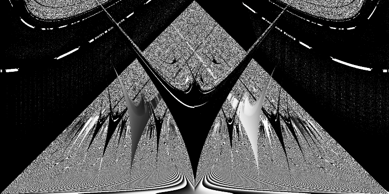
plot_phase_space(df)

Computing a Smooth Rotation Number
We now compute a smooth rotation number $\tilde{\omega}$, which we define as:
\[\tilde{\omega} = \lim_{n \to\infty} \frac{1}{n} \sum_{i=0}^n \theta_i\]This averaging method can provide different results from our previous approach in chaotic or strongly nonlinear regimes because it considers all intermediate positions rather than just the net displacement.
@jit(nopython=True, fastmath=True)
def compute_smooth_rotation_number_cpu(omega, k, num_iter):
    """
    Compute the smooth rotation number by averaging all phase values.

    Args:
        omega: Frequency ratio parameter
        k: Coupling strength parameter
        num_iter: Number of iterations for averaging

    Returns:
        Smooth rotation number
    """
    theta = 0.0
    rotation_number = 0.0
    for i in range(num_iter):
        theta = circle_map_cpu(theta, omega, k)
        rotation_number += theta / num_iter
    return rotation_number
Updated CPU Implementation with Smooth Rotation Number
We now extend our CPU implementation to support both calculation methods:
@jit(nopython=True, parallel=True, fastmath=True)
def compute_all_cpu(n_omega=1000, n_k=500, num_iter=10_000, smooth=True):
    """
    Compute rotation numbers across a parameter grid with option for smooth calculation.

    Args:
        n_omega: Number of points along the omega axis
        n_k: Number of points along the k axis
        num_iter: Number of iterations for each computation
        smooth: Whether to use the smooth rotation number calculation

    Returns:
        k_values: Array of k values
        omega_values: Array of omega values
        rotation_numbers: 2D array of rotation numbers
    """
    # Create parameter grids
    omega_values = np.linspace(0.0, 1.0, n_omega)
    k_values = np.linspace(0.0, 0.5, n_k)
    rotation_numbers = np.zeros((n_k, n_omega))

    # Choose calculation method based on smooth flag
    if smooth:
        for i in prange(n_k):
            for j in range(n_omega):
                rotation_numbers[i, j] = compute_smooth_rotation_number_cpu(
                    omega_values[j], k_values[i], num_iter
                )
    else:
        for i in prange(n_k):
            for j in range(n_omega):
                rotation_numbers[i, j] = compute_rotation_number_cpu(
                    omega_values[j], k_values[i], num_iter
                )

    return k_values, omega_values, rotation_numbers
Let’s run the computation with the smooth rotation number method:
%%time
start = perf_counter()
k_values, omega_values, rotation_numbers = compute_all_cpu(
    n_omega=2_000, n_k=1_000, num_iter=10_000
)
et_wall_cpu = perf_counter() - start
CPU times: user 15min 20s, sys: 152 ms, total: 15min 20s
Wall time: 1min 1s
As before, we prepare the data for visualization and visualize the phase space with our smooth rotation number:
df = create_dataframe(k_values, omega_values, rotation_numbers)
plot_phase_space(df)

GPU Implementation
Now let’s accelerate our computation using GPU parallelism with Numba CUDA. First, we implement the circle map function for the GPU:
@cuda.jit(device=True)
def circle_map_gpu(theta, omega, k):
    """
    Single iteration of the circle map (GPU version).

    Args:
        theta: Current phase
        omega: Frequency ratio parameter
        k: Coupling strength parameter

    Returns:
        New phase (modulo 1)
    """
    return (theta + omega + k * np.sin(2.0 * np.pi * theta)) % 1.0
Next, we create a CUDA kernel to compute the smooth rotation number:
@cuda.jit
def compute_smooth_rotation_number_kernel_gpu(
    omega_values, k_values, rotation_numbers, num_iter
):
    """
    CUDA kernel for computing smooth rotation numbers across parameter grid.

    Args:
        omega_values: Array of omega values
        k_values: Array of k values
        rotation_numbers: Output array for rotation numbers
        num_iter: Number of iterations for each computation
    """
    i, j = cuda.grid(2)
    if i < k_values.shape[0] and j < omega_values.shape[0]:
        theta = 0.0
        sum_theta = 0.0
        omega = omega_values[j]
        k = k_values[i]
        for _ in range(num_iter):
            theta = circle_map_gpu(theta, omega, k)
            sum_theta += theta / num_iter
        rotation_numbers[i, j] = sum_theta

def compute_all_gpu(n_omega=1000, n_k=500, num_iter=10_000, block_size=16):
    """
    Compute rotation numbers across a parameter grid using GPU acceleration.

    Args:
        n_omega: Number of points along the omega axis
        n_k: Number of points along the k axis
        num_iter: Number of iterations for each computation
        block_size: Size of CUDA thread blocks

    Returns:
        k_values: Array of k values
        omega_values: Array of omega values
        rotation_numbers: 2D array of rotation numbers
    """
    # Create parameter grids
    omega_values = np.linspace(0.0, 1.0, n_omega).astype(np.float32)
    k_values = np.linspace(0.0, 0.5, n_k).astype(np.float32)
    rotation_numbers = np.zeros((n_k, n_omega), dtype=np.float32)

    # Transfer these arrays to the GPU device memory
    d_omega_values = cuda.to_device(omega_values)
    d_k_values = cuda.to_device(k_values)
    d_rotation_numbers = cuda.to_device(rotation_numbers)

    # CUDA organizes parallel execution using blocks of threads, which run on a grid.
    threads_per_block = (block_size, block_size)
    blocks_per_grid_x = (n_k + threads_per_block[0] - 1) // threads_per_block[0]
    blocks_per_grid_y = (n_omega + threads_per_block[1] - 1) // threads_per_block[1]
    blocks_per_grid = (blocks_per_grid_x, blocks_per_grid_y)

    # Launch the kernel
    compute_smooth_rotation_number_kernel_gpu[blocks_per_grid, threads_per_block](
        d_omega_values, d_k_values, d_rotation_numbers, num_iter
    )

    # Copy the computed rotation number results back to the host memory
    rotation_numbers = d_rotation_numbers.copy_to_host()

    return k_values, omega_values, rotation_numbers
Let’s run the GPU computation with the same parameters as our CPU version:
%%time
start = perf_counter()
k_values, omega_values, rotation_numbers = compute_all_gpu(
    n_omega=2_000, n_k=1_000, num_iter=10_000
)
et_wall_gpu = perf_counter() - start
CPU times: user 6.52 s, sys: 176 ms, total: 6.69 s
Wall time: 6.72 s
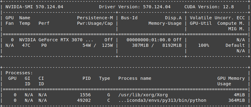
A screenshot of nvidia-smi during execution shows the GPU utilization:

df = create_dataframe(k_values, omega_values, rotation_numbers)
plot_phase_space(df)

GPU Performance Speedup
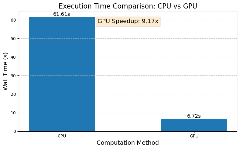
Let’s visualize the performance comparison between our CPU and GPU implementations:
methods = ["CPU", "GPU"]
execution_times = [et_wall_cpu, et_wall_gpu]
fig, ax = plt.subplots(figsize=(8, 5))
bars = ax.bar(methods, execution_times, width=0.5)
ax.set_title("Execution Time Comparison: CPU vs GPU", fontsize=16)
ax.set_xlabel("Computation Method", fontsize=14)
ax.set_ylabel("Wall Time (s)", fontsize=14)
for bar in bars:
    height = bar.get_height()
    ax.text(
        bar.get_x() + bar.get_width() / 2.0,
        height + 0.1,
        f"{height:.2f}s",
        ha="center",
        va="bottom",
        fontsize=12,
    )
ax.grid(axis="y", linestyle="--", alpha=0.7)
speedup = et_wall_cpu / et_wall_gpu
_ = ax.text(
    0.5,
    0.9,
    f"GPU Speedup: {speedup:.2f}x",
    horizontalalignment="center",
    transform=ax.transAxes,
    fontsize=14,
    bbox=dict(facecolor="#f39c12", alpha=0.2),
)
plt.tight_layout()

High-Resolution Arnold Tongues with CUDA
Using Numba-CUDA acceleration, we can generate detailed visualizations by increasing the resolution of our parameter grid:
%%time
k_values, omega_values, rotation_numbers = compute_all_gpu(
    n_omega=20_000, n_k=10_000, num_iter=10_000
)
CPU times: user 10min 32s, sys: 609 ms, total: 10min 33s
Wall time: 10min 33s
Even with 200 million parameter combinations (20,000 × 10,000) and 10,000 iterations per parameter couple, the GPU computation completes in 10 minutes.
%%time
df = create_dataframe(k_values, omega_values, rotation_numbers)
plot_phase_space(df, size_x=2_000, size_y=1_000)
CPU times: user 9.2 s, sys: 6.89 s, total: 16.1 s
Wall time: 16.5 s
