Zipf's Law on "La Comédie humaine"

In this Python notebook, we’re going to explore Zipf’s law as applied to words.

Zipf’s law is an empirical law stating that when a list of measured values is sorted in decreasing order, the value of the n-th entry is often approximately inversely proportional to n.

This is the definition of Zipf’s law from its wikipedia page. One of the most famous observation of Zipf’s law is from word distribution in a text corpus. It can be expressed as:

\[f(r) \propto \frac{1}{r}\]

Where:

• $f(r)$ is the frequency of a word with rank $r$
• $r$ is the rank of the word when all words are arranged by decreasing frequency

It’s worth noting that this law was first investigated by the French stenographer Jean-Baptiste Estoup (left/top) in 1916 and later extended and widely popularized by the American linguist George Kingsley Zipf (right/bottom).

This low applied to words may suggest that language follows a principle of least effort, where communicators balance the desire for precision ($r$ is large) with efficiency ($r$ is small). Zipf wrote:

The power laws in linguistics and in other human systems reflect an economical rule: everything carried out by human beings and other biological entities must be done with least effort (at least statistically)

More generally, the relationship is written as:

\[f(r) = \frac{C}{r^{\alpha}}\]

Where:

• $C$ is a normalizing constant
• $\alpha$ is an exponent that characterizes the distribution, usually close to 1

In a log-log plot, Zipf’s law appears as a straight line with slope $-\alpha$:

\[\log(f(r)) = \log(C) - \alpha \log(r)\]

Let’s check how this applies to a text corpus. For this, we are using Honoré de Balzac’s extensive series of books called “La Comédie Humaine” (in French). It’s a collection of many novels depicting French society, written between 1829 and 1850.

Here is the outline of the post:

• Imports and package versions
• Scrape Project Gutenberg
• Download the books
• Create a corpus
• Analyze word frequencies

Imports and package versions

import glob
import os
import re
import time
from collections import Counter

import matplotlib.pyplot as plt
import numpy as np
import pandas as pd
import requests
import tol_colors
from bs4 import BeautifulSoup
from sklearn.linear_model import LinearRegression
from sklearn.preprocessing import StandardScaler
from slugify import slugify

tol_colors.set_default_colors()

OUTPUT_DP = "./balzac_comedie_humaine"  # output dir path

Package versions:

Python implementation: CPython
Python version       : 3.13.3

matplotlib: 3.10.3
numpy     : 2.2.5
pandas    : 2.2.3
requests  : 2.32.3
tol_colors: 2.0.0
bs4       : 4.13.4
sklearn   : 1.6.1
slugify   : 8.0.4

Scrape Project Gutenberg

We want to scrape Project Gutenberg’s French language page to find Balzac’s La Comédie humaine volumes. Since the series consists of 17 volumes, we’ll use BeautifulSoup to automatically extract their titles and IDs from the webpage.

URL = "https://www.gutenberg.org/browse/languages/fr"
response = requests.get(URL)
soup = BeautifulSoup(response.text, "html.parser")

# locate Balzac's section
balzac_h2 = None
for h2 in soup.find_all("h2"):
    if "Balzac, Honoré de" in h2.text:
        balzac_h2 = h2
        break

v = {}
book_list = balzac_h2.find_next("ul")
for book_li in book_list.find_all("li", class_="pgdbetext"):

    link = book_li.find("a")
    if not link or not link.has_attr("href"):
        continue

    title = link.text.strip()
    if not title.startswith("La Comédie humaine - Volume"):
        continue

    # book ID
    book_id_match = re.search(r"/ebooks/(\d+)", link["href"])
    if not book_id_match:
        continue

    book_id = book_id_match.group(1)
    v[title] = book_id

volumes = pd.DataFrame(list(v.items()), columns=["title", "pg_id"])
volumes.head(3)

	title	pg_id
0	La Comédie humaine - Volume 01	41211
1	La Comédie humaine - Volume 02	43851
2	La Comédie humaine - Volume 03	45060

volumes.shape

(17, 2)

We’ve successfully extracted all 17 volumes. The Project Gutemberg book ID pg_id is what we need to later be able to download the books. Let’s also extract the volume number from the title to ensure that we process them in the correct order:

def extract_volume_number(title):
    match = re.search(r"Volume\s+(\d+)", title)
    if match:
        return int(match.group(1))
    return -1


volumes["volume"] = volumes.title.map(extract_volume_number)
volumes = volumes.sort_values(by="volume")
volumes.head(3)

	title	pg_id	volume
0	La Comédie humaine - Volume 01	41211	1
1	La Comédie humaine - Volume 02	43851	2
2	La Comédie humaine - Volume 03	45060	3

Download the books

First we sanitize the titles to create file names that are file-system friendly:

volumes["filename"] = volumes["title"].map(lambda s: f"{slugify(s)}.txt")
volumes.head(3)

	title	pg_id	volume	filename
0	La Comédie humaine - Volume 01	41211	1	la-comedie-humaine-volume-01.txt
1	La Comédie humaine - Volume 02	43851	2	la-comedie-humaine-volume-02.txt
2	La Comédie humaine - Volume 03	45060	3	la-comedie-humaine-volume-03.txt

We create the output directory if it doesn’t exist.

if not os.path.exists(OUTPUT_DP):
    os.makedirs(OUTPUT_DP)

Let’s use a small downloading function. It returns True when a web request has been made, which then triggers a 2-seconds pause to limit the requests rate:

def download_book(book_id, title, filename, output_dir="balzac_comedie_humaine"):
    filepath = os.path.join(output_dir, filename)
    if os.path.exists(filepath):
        print(f"Skipping already downloaded: {title}")
        return False

    url = f"https://www.gutenberg.org/cache/epub/{book_id}/pg{book_id}.txt"
    print(f"Downloading: {title} (ID: {book_id})")
    try:
        response = requests.get(url)
        if response.status_code == 200:
            with open(filepath, "wb") as f:
                f.write(response.content)
            print(f"Saved to {filepath}")
    except Exception as e:
        print(f"Failed to download {title}")
        print(e)
    return True

Now let’s download all 17 volumes in sequence:

%%time
for row in volumes.itertuples():
    title = row.title
    book_id = row.pg_id
    filename = row.filename
    if download_book(book_id, title, filename, output_dir=OUTPUT_DP):
        time.sleep(2)

Downloading: La Comédie humaine - Volume 01 (ID: 41211)
Saved to ./balzac_comedie_humaine/la-comedie-humaine-volume-01.txt
Downloading: La Comédie humaine - Volume 02 (ID: 43851)
Saved to ./balzac_comedie_humaine/la-comedie-humaine-volume-02.txt
Downloading: La Comédie humaine - Volume 03 (ID: 45060)
Saved to ./balzac_comedie_humaine/la-comedie-humaine-volume-03.txt
Downloading: La Comédie humaine - Volume 04 (ID: 48082)
Saved to ./balzac_comedie_humaine/la-comedie-humaine-volume-04.txt
Downloading: La Comédie humaine - Volume 05. Scènes de la vie de Province - Tome 01 (ID: 49482)
Saved to ./balzac_comedie_humaine/la-comedie-humaine-volume-05-scenes-de-la-vie-de-province-tome-01.txt
Downloading: La Comédie humaine - Volume 06. Scènes de la vie de Province - Tome 02 (ID: 51381)
Saved to ./balzac_comedie_humaine/la-comedie-humaine-volume-06-scenes-de-la-vie-de-province-tome-02.txt
Downloading: La Comédie humaine - Volume 07. Scènes de la vie de Province - Tome 03 (ID: 52831)
Saved to ./balzac_comedie_humaine/la-comedie-humaine-volume-07-scenes-de-la-vie-de-province-tome-03.txt
Downloading: La Comédie humaine - Volume 08. Scènes de la vie de Province - Tome 04 (ID: 54723)
Saved to ./balzac_comedie_humaine/la-comedie-humaine-volume-08-scenes-de-la-vie-de-province-tome-04.txt
Downloading: La Comédie humaine - Volume 09. Scènes de la vie parisienne - Tome 01 (ID: 55860)
Saved to ./balzac_comedie_humaine/la-comedie-humaine-volume-09-scenes-de-la-vie-parisienne-tome-01.txt
Downloading: La Comédie humaine - Volume 10. Scènes de la vie parisienne - Tome 02 (ID: 58244)
Saved to ./balzac_comedie_humaine/la-comedie-humaine-volume-10-scenes-de-la-vie-parisienne-tome-02.txt
Downloading: La Comédie humaine - Volume 11. Scènes de la vie parisienne - Tome 03 (ID: 60551)
Saved to ./balzac_comedie_humaine/la-comedie-humaine-volume-11-scenes-de-la-vie-parisienne-tome-03.txt
Downloading: La Comédie humaine - Volume 12. Scènes de la vie parisienne et scènes de la vie politique (ID: 67264)
Saved to ./balzac_comedie_humaine/la-comedie-humaine-volume-12-scenes-de-la-vie-parisienne-et-scenes-de-la-vie-politique.txt
Downloading: La Comédie humaine - Volume 13. Scènes de la vie militaire et Scènes de la vie de campagne (ID: 71022)
Saved to ./balzac_comedie_humaine/la-comedie-humaine-volume-13-scenes-de-la-vie-militaire-et-scenes-de-la-vie-de-campagne.txt
Downloading: La Comédie humaine - Volume 14. Études philosophiques (ID: 71773)
Saved to ./balzac_comedie_humaine/la-comedie-humaine-volume-14-etudes-philosophiques.txt
Downloading: La Comédie humaine - Volume 15. Études philosophiques (ID: 72034)
Saved to ./balzac_comedie_humaine/la-comedie-humaine-volume-15-etudes-philosophiques.txt
Downloading: La Comédie humaine - Volume 16. Études philosophiques et Études analytiques (ID: 73552)
Saved to ./balzac_comedie_humaine/la-comedie-humaine-volume-16-etudes-philosophiques-et-etudes-analytiques.txt
Downloading: La Comédie humaine - Volume 17. Études de mœurs :  La cousine Bette; Le cousin Pons (ID: 74126)
Saved to ./balzac_comedie_humaine/la-comedie-humaine-volume-17-etudes-de-moeurs-la-cousine-bette-le-cousin-pons.txt
CPU times: user 622 ms, sys: 224 ms, total: 846 ms
Wall time: 52.8 s

Create a corpus

Now that we have all the text files downloaded, we need to load and combine them into a single corpus for analysis.

file_pattern = os.path.join(OUTPUT_DP, "*.txt")
files = glob.glob(file_pattern)
files.sort()
assert len(files) == volumes.shape[0]

Let’s read each file into memory.

texts = {}
for file_path in files:
    file_name = os.path.basename(file_path)
    try:
        with open(file_path, "r", encoding="utf-8") as file:
            content = file.read()
            texts[file_name] = content
            print(f"Loaded: {file_name}")
    except Exception as e:
        print(f"Error loading {file_name}: {str(e)}")

print(f"Successfully loaded {len(texts)} files.")

Loaded: la-comedie-humaine-volume-01.txt
Loaded: la-comedie-humaine-volume-02.txt
Loaded: la-comedie-humaine-volume-03.txt
Loaded: la-comedie-humaine-volume-04.txt
Loaded: la-comedie-humaine-volume-05-scenes-de-la-vie-de-province-tome-01.txt
Loaded: la-comedie-humaine-volume-06-scenes-de-la-vie-de-province-tome-02.txt
Loaded: la-comedie-humaine-volume-07-scenes-de-la-vie-de-province-tome-03.txt
Loaded: la-comedie-humaine-volume-08-scenes-de-la-vie-de-province-tome-04.txt
Loaded: la-comedie-humaine-volume-09-scenes-de-la-vie-parisienne-tome-01.txt
Loaded: la-comedie-humaine-volume-10-scenes-de-la-vie-parisienne-tome-02.txt
Loaded: la-comedie-humaine-volume-11-scenes-de-la-vie-parisienne-tome-03.txt
Loaded: la-comedie-humaine-volume-12-scenes-de-la-vie-parisienne-et-scenes-de-la-vie-politique.txt
Loaded: la-comedie-humaine-volume-13-scenes-de-la-vie-militaire-et-scenes-de-la-vie-de-campagne.txt
Loaded: la-comedie-humaine-volume-14-etudes-philosophiques.txt
Loaded: la-comedie-humaine-volume-15-etudes-philosophiques.txt
Loaded: la-comedie-humaine-volume-16-etudes-philosophiques-et-etudes-analytiques.txt
Loaded: la-comedie-humaine-volume-17-etudes-de-moeurs-la-cousine-bette-le-cousin-pons.txt
Successfully loaded 17 files.

Before analyzing the word frequencies, we need to preprocess the text to remove Project Gutenberg headers and normalize the text:

def preprocess_text(text):

    # remove Project Gutenberg header and footer
    start_marker = "*** START OF THIS PROJECT GUTENBERG EBOOK"
    end_marker = "*** END OF THIS PROJECT GUTENBERG EBOOK"

    if start_marker in text:
        text = text.split(start_marker)[1]
    if end_marker in text:
        text = text.split(end_marker)[0]

    # convert to lowercase
    text = text.lower()

    # remove special characters and numbers
    text = re.sub(r"[^\w\s]", " ", text)
    text = re.sub(r"\d+", " ", text)

    # remove multiple spaces
    text = re.sub(r"\s+", " ", text)

    return text.strip()

Now let’s combine all volumes into a single corpus:

corpus = ""
for item in texts.values():
    text = preprocess_text(item)
    corpus += text + "\n"

We check the size of our final corpus:

print(f"Length of preprocessed corpus: {len(corpus)} characters")

Length of preprocessed corpus: 22087522 characters

Analyze word frequencies

We start by counting each word’s occurrences and sort the words by their frequency:

words = text.split()
word_counts = Counter(words)

freq = pd.DataFrame(
    {"word": list(word_counts.keys()), "frequency": list(word_counts.values())}
)
freq = freq.sort_values("frequency", ascending=False).reset_index(drop=True)
freq["rank"] = freq.index + 1
freq["log_frequency"] = np.log10(freq["frequency"])
freq["log_rank"] = np.log10(freq["rank"])
print(freq.head(10))

  word  frequency  rank  log_frequency  log_rank
0   de      10964     1       4.039969  0.000000
1   la       7412     2       3.869935  0.301030
2   le       6246     3       3.795602  0.477121
3    à       5161     4       3.712734  0.602060
4   et       5119     5       3.709185  0.698970
5  les       3916     6       3.592843  0.778151
6    l       3846     7       3.585009  0.845098
7   en       3722     8       3.570776  0.903090
8   il       3543     9       3.549371  0.954243
9   un       3478    10       3.541330  1.000000

Remark : we are keeping stop words in the dictionary.

freq.shape

(19963, 5)

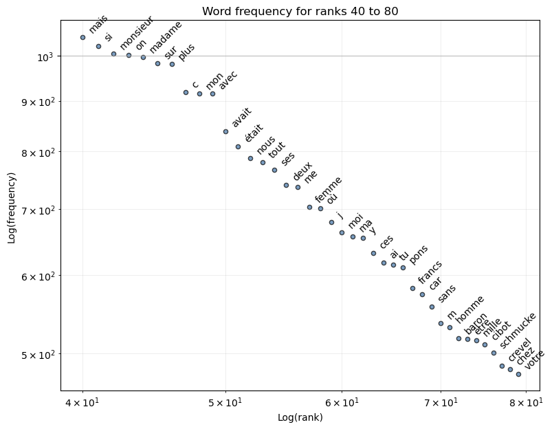
We have a “vocabulary” size of around 20000 words. This gives us a dataset large enough to observe Zipf’s law. Let’s create a visualization function to explore frequencies across different rank ranges:

def plot_limited_frequencies(freq, rank_start=1, rank_end=11):
    selected_words = freq.iloc[rank_start-1:rank_end-1]
    ax = selected_words.plot.scatter(
        "rank", "frequency", alpha=0.7, edgecolors="k", figsize=(9, 7)
    )
    ax.set_xscale("log")
    ax.set_yscale("log")
    ax.grid(True)
    ax.set(
        title=f"Word frequency for ranks {rank_start} to {rank_end}",
        xlabel="Log(rank)",
        ylabel="Log(frequency)",
    )    
    for i, row in selected_words.iterrows():
        plt.annotate(
            row["word"],
            xy=(row["rank"], row["frequency"]),
            xytext=(5, 5),
            textcoords="offset points",
            rotation=45,
        )
    plt.grid(True, which="both", linestyle="-", linewidth=0.5, alpha=0.3)
    plt.grid(True, which="major", linestyle="-", linewidth=1, alpha=0.7)
    return ax

ax = plot_limited_frequencies(freq, 40, 80)

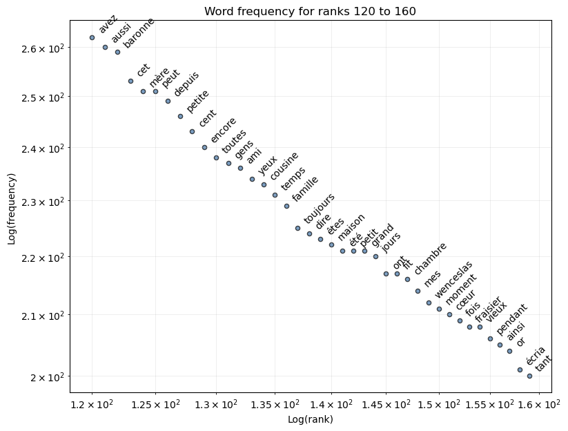
ax = plot_limited_frequencies(freq, 120, 160)

Let’s visualize Zipf’s law with all the words and add a linear regression. Note that we use a weighted regression with weights proportional to the word frequencies. When working with Zipf’s law in log-log space, the regression can indeed be disproportionately influenced by the long tail of less frequent words.

plt.figure(figsize=(8, 6))
plt.plot(
    freq["log_rank"],
    freq["log_frequency"],
    "o-",
    ms=3,
    alpha=0.5,
    color="C0",
    label="Word frequency",
)

# give more importance to frequent words
weights = freq["frequency"]

# linear regression to evaluate the slope
scaler = StandardScaler()
reg = LinearRegression(fit_intercept=True)
X, y = freq[["log_rank"]].values, freq["log_frequency"].values
X_scaled = scaler.fit_transform(X)
reg.fit(X_scaled, y, sample_weight=weights)
slope_scaled = reg.coef_[0]
slope = slope_scaled / scaler.scale_[0]
intercept = reg.intercept_
r_value = reg.score(X_scaled, y, sample_weight=weights)

x_orig = np.linspace(freq["log_rank"].min(), freq["log_rank"].max(), 100)
x_orig_2d = x_orig.reshape(-1, 1)
x_scaled = scaler.transform(x_orig_2d).flatten()
y_pred = slope_scaled * x_scaled + intercept

plt.plot(
    x_orig,
    y_pred,
    "-",
    label=f"Regression slope: {slope:.3f}, R²: {r_value:.3f}",
    color="C1",
)

plt.xlabel("Log(rank)")
plt.ylabel("Log(frequency)")
plt.title("""Zipf's law applied to "La Comédie humaine" by Honoré de Balzac""")
plt.legend()
plt.grid(True)

plt.tight_layout()

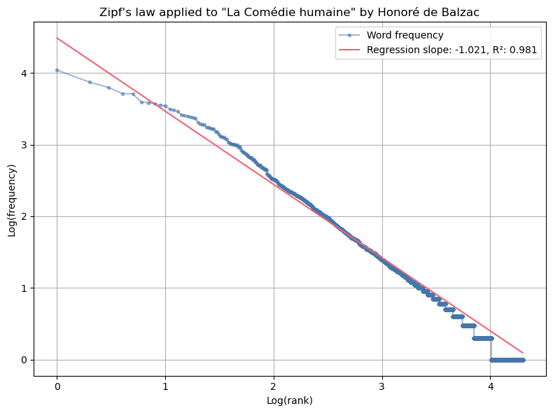
Looking at the visualization, we can observe that Zipf’s law doesn’t fit very well for the highest-ranked words (“de”, “la”, “le”, “à”, “et”, …). The most frequent words tend to be less frequent than what the simple power law predicts. And because we gave these words the largest weights in the regression, this deteriorates the fit. Maybe the Zipf-Mandelbrot law might provide a better fit. It is a more general formula that includes an additional parameter:

\[f(r) = \frac{C}{(r + q)^{\alpha}}\]

where $q$ is an additional parameter that effectively shifts the rank, allowing the model to better account for the behavior of the most frequent words.