Computing and Visualizing Billions of Bohemian Eigenvalues with Python
According to www.bohemianmatrices.com/,
A family of Bohemian matrices is a distribution of random matrices where the matrix entries are sampled from a discrete set of bounded height. The discrete set must be independent of the dimension of the matrices.
In our case, we sample 5x5 matrix entries from the discrete set {-1, 0, 1}. For example, here are 2 random matrices with these specifications:
\[\begin{pmatrix} 0 & 0 & 0 & -1 & 0 \\ 0 & 0 & 0 & 1 & -1 \\ 1 & -1 & 0 & -1 & -1 \\ 1 & -1 & 1 & 1 & 0 \\ -1 & 0 & 1 & 0 & -1 \end{pmatrix}\] \[\begin{pmatrix} -1 & 0 & 0 & 0 & 0 \\ 0 & 1 & 0 & 1 & 1 \\ 1 & -1 & 0 & -1 & -1 \\ 1 & 1 & 1 & 1 & -1 \\ -1 & 0 & 1 & -1 & -1 \end{pmatrix}\]Bohemian eigenvalues are the eigenvalues of a family of Bohemian matrices. Eigenvalues $λ$ satisfy the equation $Av = λv$, where $A$ is the matrix and $v$ is a corresponding eigenvector. If the matrices are 5 by 5, the eigenvalue solver is going to return 5 complex eigenvalues.
So what if we want to compute all the possible eigenvalues from all these matrices? Well that would imply $3^{5 \times 5} = 847,288,609,443$ matrices, resulting in $4.236 × 10^{12}$ eigenvalues. Just storing all these matrices would require some significant space. Each 5×5 matrix has 25 entries, and if we need 1 byte per entry to represent {-1, 0, 1}, we get a total storage amount of : $847,288,609,443$ matrices × 25 bytes/matrix = $21,182,215,236,075$ bytes ≈ 21.18 TB
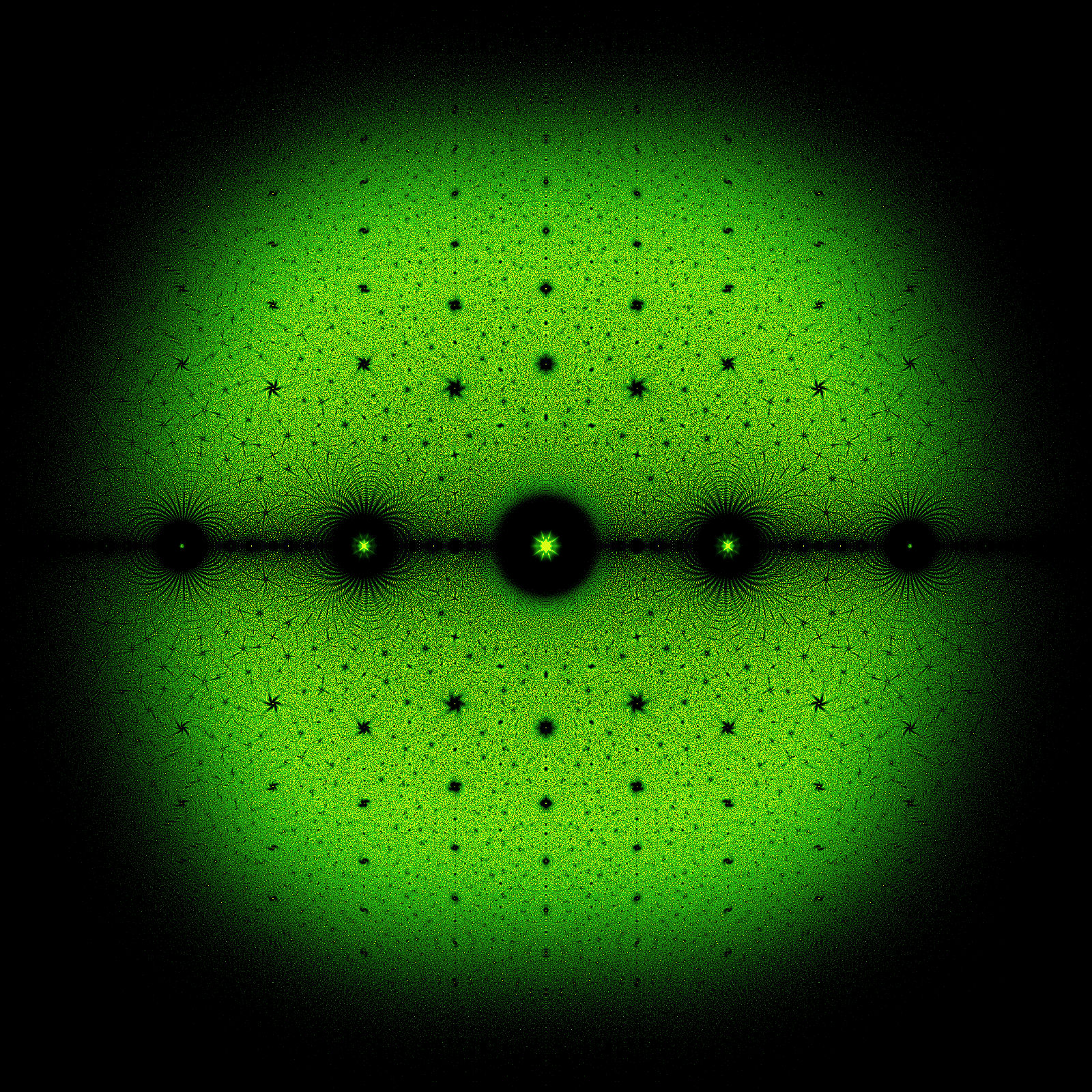
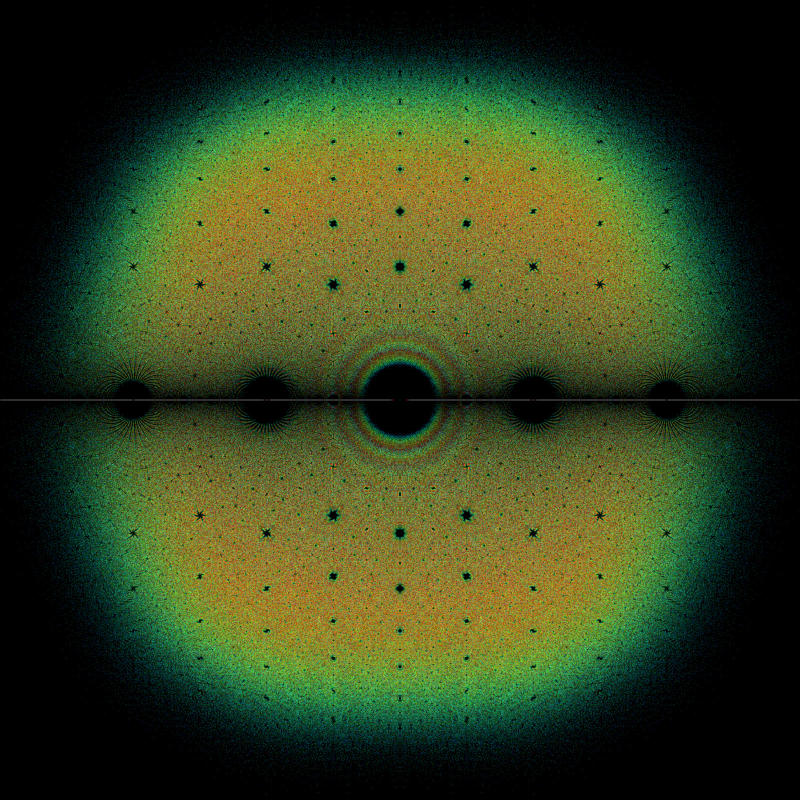
So instead of computing all possible matrices, we are only going to sample 1 billion matrices. The first motivation to compute these complex eigenvalues is to observe some interesting patterns when plotted in the complex plane. See for example the beautiful gallery from the bohemianmatrices web site : www.bohemianmatrices.com/gallery/. Actually, we are just going to reproduce one of the gallery images :
Although I like the resulting plot, the main point of this Python notebook is to be able to compute and visualize these 5 billion eigenvalues smoothly. My laptop has 32GB of RAM and a 20-cores Intel i9 CPU. And for that, we are going to use some great packages: numpy, numba, pyarrow, dask and datashader. Note that I tried to perform the eigenvalue computations with PyTorch on my GPU but it did not improve the overall efficiency for these very small matrices as compared to numba.
We are going to process by batch for the eigenvalues computation and the visualization. This workflow has two distinct steps:
-
Generate, compute and store: We generate matrices in batches, compute eigenvalues in parallel using Numba’s
njit, and write the eigenvalues incrementally to a Parquet file. -
Load and visualize: We use dask to load data from the Parquet file in chunks, distributing points into partition buckets for out-of-core visualization with Datashader.
This chunk approach allows us to process billions of eigenvalues without overwhelming system memory.
Package versions
Python implementation: CPython
Python version       : 3.13.3

dask      : 2025.5.0
datashader: 0.18.1
numpy     : 2.2.6
pyarrow   : 20.0.0
colorcet  : 3.1.0
numba     : 0.61.2
tqdm      : 4.67.1
First Part : computing eigenvalues in batches
import gc
import os

import numpy as np
import pyarrow as pa
import pyarrow.parquet as pq
from numba import njit, prange
from tqdm import tqdm

PARQUET_FP = "./eigenvalues.parquet"
RS = 124
@njit(parallel=True, fastmath=True)
def compute_eigenvalues_batch(entries, indices, mat_size):
    batch_size = indices.shape[0] // (mat_size * mat_size)
    eigs = np.empty(batch_size * mat_size, dtype=np.complex64)
    for i in prange(batch_size):
        mat = np.empty((mat_size, mat_size), dtype=np.complex64)
        for j in range(mat_size):
            for k in range(mat_size):
                index = indices[i * mat_size * mat_size + j * mat_size + k]
                mat[j, k] = entries[index]
        start = i * mat_size
        eigs[start : start + mat_size] = np.linalg.eigvals(mat)
    return eigs

def compute_and_save_eigenvalues(
    output_path, entries, mat_size, total_count, batch_size, seed=42
):
    np.random.seed(seed)
    entries_array = np.array(entries, dtype=np.float32)
    num_choices = len(entries)
    schema = pa.schema(
        [
            ("x", pa.float32()),
            ("y", pa.float32()),
        ]
    )
    with pq.ParquetWriter(output_path, schema) as writer:
        for offset in tqdm(range(0, total_count, batch_size)):
            current_batch = min(batch_size, total_count - offset)
            num_elements = current_batch * mat_size * mat_size
            random_indices = np.random.randint(
                0, num_choices, size=num_elements
            ).astype(np.uint8)
            eigvals = compute_eigenvalues_batch(entries_array, random_indices, mat_size)
            table = pa.table(
                {
                    "x": eigvals.real.astype(np.float32),
                    "y": eigvals.imag.astype(np.float32),
                },
                schema=schema,
            )
            writer.write_table(table)
            del eigvals, table
            gc.collect()
We remove the parquet file if it’s already there:
if os.path.exists(PARQUET_FP):
    os.remove(PARQUET_FP)
    print(f"Deleted: {PARQUET_FP}")
else:
    print(f"File does not exist: {PARQUET_FP}")
File does not exist: ./eigenvalues.parquet
Let’s generate 1 billion 5×5 matrices with entries from {-1, 0, 1} and compute their eigenvalues by batch of 10,000,000:
%%time

compute_and_save_eigenvalues(
    output_path=PARQUET_FP,
    entries=[-1, 0, 1],
    mat_size=5,
    total_count=1_000_000_000,
    batch_size=10_000_000,
    seed=RS,
)
100%|█████████████████████████████████████████████████████████████████████████████████████████████████████████████████████████████████████████| 100/100 [19:49<00:00, 11.90s/it]

CPU times: user 4h 14min 28s, sys: 1min 22s, total: 4h 15min 51s
Wall time: 19min 49s
Second part : visualization with Datashader
Datashader handles large datasets efficiently when used with dask by processing data in chunks and creating density plots without loading all points into memory, only the final raster (the image) is kept in memory.
import dask.dataframe as dd
import datashader as ds
import datashader.transfer_functions as tf
from datashader import reductions as rd
from colorcet import palette

cmap = palette["kgy"]
bg_col = "black"
We filter out real eigenvalues located near the real axis (those with imaginary part magnitude smaller than eps) to focus on the complex structure. We also remove potential eigenvalues outside the square box $-3\leq x\leq3$ and $-3\leq y\leq3$. The max_points parameter caps pixel density values to prevent oversaturation.
def visualize(
    parquet_path,
    plot_width=1600,
    plot_height=1600,
    x_range=(-3, 3),
    y_range=(-3, 3),
    eps=1e-5,
    cmap="fire",
    bg_col="black",
    output_path="output.png",
    how="log",
    max_points=1000
):
    ddf = dd.read_parquet(parquet_path, columns=["x", "y"])
    nrows, ncols = ddf.shape[0].compute(), ddf.shape[1]
    print(f"Before filtering : {nrows} rows, {ncols} columns")
    ddf = ddf[
        (ddf["x"] >= x_range[0])
        & (ddf["x"] <= x_range[1])
        & (ddf["y"] >= y_range[0])
        & (ddf["y"] <= y_range[1])
        & ((ddf["y"] <= -eps) | (ddf["y"] >= eps))
    ]
    nrows, ncols = ddf.shape[0].compute(), ddf.shape[1]
    print(f"After filtering : {nrows} rows, {ncols} columns")
    cvs = ds.Canvas(
        plot_width=plot_width, plot_height=plot_height, x_range=x_range, y_range=y_range
    )
    agg = cvs.points(ddf, "x", "y", agg=rd.count())
    agg_capped = agg.where(agg <= max_points, max_points)
    img = tf.shade(agg_capped, cmap=cmap, how=how)
    img = tf.set_background(img, bg_col)
    img.to_pil().save(output_path)
    return img
%%time

visualize(
    parquet_path=PARQUET_FP,
    cmap=cmap,
    bg_col=bg_col,
    output_path="bohemian_01.png",
    eps=1e-3,
    how="eq_hist",
    max_points=2000
)
Before filtering : 5000000000 rows, 2 columns
After filtering : 2640645434 rows, 2 columns
CPU times: user 9min 15s, sys: 11min 16s, total: 20min 31s
Wall time: 1min 45s