A Git commit temporal analysis
In this Python notebook, we are going to analyze git commit timestamps across multiple repositories to identify temporal patterns in a git user coding activity (me, actually).
Outline
Imports and Package Versions
BASE_DIR is the root folder containing all the git repositories. The USER_FILTERS list contains substrings to match against git author names for filtering commits from a specific user with various names (github, gitlab from various organizations). You can adapt these two variables with your own directory and git user names.
import os
import subprocess
from collections import Counter
from datetime import datetime

import matplotlib.pyplot as plt
import numpy as np
import pandas as pd
import tol_colors as tc

BASE_DIR = "/home/francois/Workspace"
USER_FILTERS = ["pacull", "djfrancesco"]
We are using Python 3.13.3 on a Linux OS:
pandas    : 2.2.3
numpy     : 2.2.6
matplotlib: 3.10.3
tol_colors: 2.0.0
Repository discovery and data extraction
Here we introduce functions to recursively scan directories for git repositories, extract commit metadata using git log in a Python subprocess, specifically commit timestamps and author names, and filter commits by author name using case-insensitive substring matching.
def is_git_repo(path):
    return os.path.isdir(os.path.join(path, ".git"))


def get_all_git_repos(base_dir):
    git_repos = []
    for root, dirs, files in os.walk(base_dir):
        if is_git_repo(root):
            git_repos.append(root)
            dirs.clear()
    return git_repos


def get_commits(repo_path):
    try:
        result = subprocess.run(
            ["git", "-C", repo_path, "log", "--pretty=format:%an|%aI"],
            stdout=subprocess.PIPE,
            stderr=subprocess.DEVNULL,
            check=True,
            text=True,
        )
        lines = result.stdout.strip().split("\n")
        filtered_lines = []
        for line in lines:
            if line:
                author = line.split("|")[0].lower()
                if any(u.lower() in author for u in USER_FILTERS):
                    filtered_lines.append(line)
        return filtered_lines
    except subprocess.CalledProcessError:
        return []


def parse_commit_times(commit_lines):
    hours = []
    weekdays = []
    for line in commit_lines:
        author, iso_date = line.split("|")
        dt = datetime.fromisoformat(iso_date)
        hours.append(dt.hour)
        weekdays.append(dt.strftime("%A"))
    return hours, weekdays
Data collection
So let’s use these previous functions to iterate through the repositories, extract commit timestamps and parse them into hour-of-day and weekday components.
all_hours = []
all_weekdays = []

repos = get_all_git_repos(BASE_DIR)
for repo in repos:
    commits = get_commits(repo)
    hours, weekdays = parse_commit_times(commits)
    all_hours.extend(hours)
    all_weekdays.extend(weekdays)

print(f"Total commits found: {len(all_hours)}")
Total commits found: 7605
Data preprocessing
Now we convert the extracted data and create frequency dataframes for each hour of the day or day of the week.
hour_counts = Counter(all_hours)
hour_df = pd.DataFrame(
    {
        "hour": list(range(24)),
        "commit_count": [hour_counts.get(h, 0) for h in range(24)],
    }
)
hour_df = hour_df.set_index("hour")
hour_df["distrib"] = hour_df["commit_count"] / hour_df["commit_count"].sum()

days_order = [
    "Monday",
    "Tuesday",
    "Wednesday",
    "Thursday",
    "Friday",
    "Saturday",
    "Sunday",
]
weekday_counts = Counter(all_weekdays)
weekday_df = pd.DataFrame(
    {
        "weekday": days_order,
        "commit_count": [weekday_counts.get(day, 0) for day in days_order],
    }
)
weekday_df = weekday_df.set_index("weekday")
weekday_df["distrib"] = weekday_df["commit_count"] / weekday_df["commit_count"].sum()
hour_df.head(3)
| commit_count | distrib | |
|---|---|---|
| hour | ||
| 0 | 12 | 0.001578 |
| 1 | 3 | 0.000394 |
| 2 | 0 | 0.000000 |
assert hour_df.distrib.sum() == 1.0
weekday_df.head(3)
| commit_count | distrib | |
|---|---|---|
| weekday | ||
| Monday | 1527 | 0.200789 |
| Tuesday | 1264 | 0.166206 |
| Wednesday | 1291 | 0.169757 |
assert weekday_df.distrib.sum() == 1.0
Visualizations
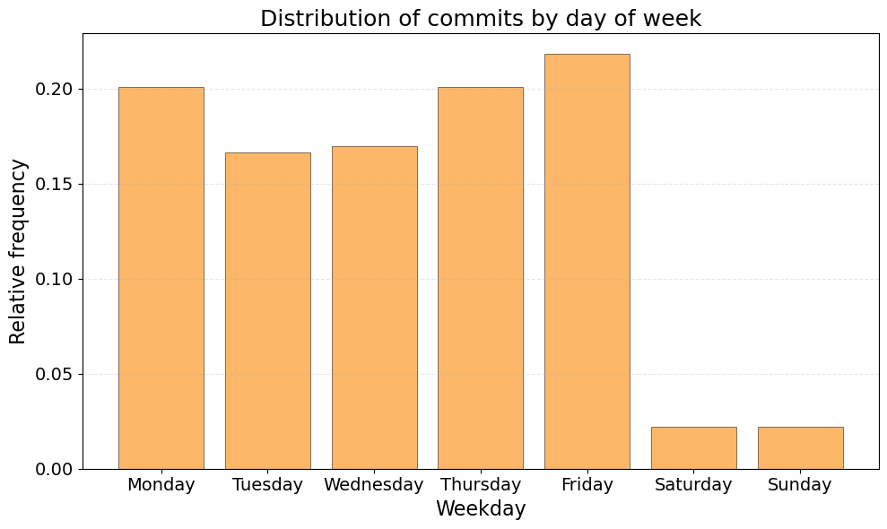
Weekly distribution
Here we create a bar chart showing normalized commit frequency across days of the week.
plt.figure(figsize=(10, 6))
colormap = tc.YlOrBr
color = colormap(0.5)
plt.bar(
    weekday_df.index,
    weekday_df["distrib"],
    color=color,
    alpha=0.7,
    edgecolor="black",
    linewidth=0.5,
)
plt.title("Distribution of commits by day of week", fontsize=18)
plt.xlabel("Weekday", fontsize=16)
plt.ylabel("Relative frequency", fontsize=16)
plt.tick_params(axis="both", labelsize=14)
plt.grid(axis="y", linestyle="--", alpha=0.3)
plt.tight_layout()
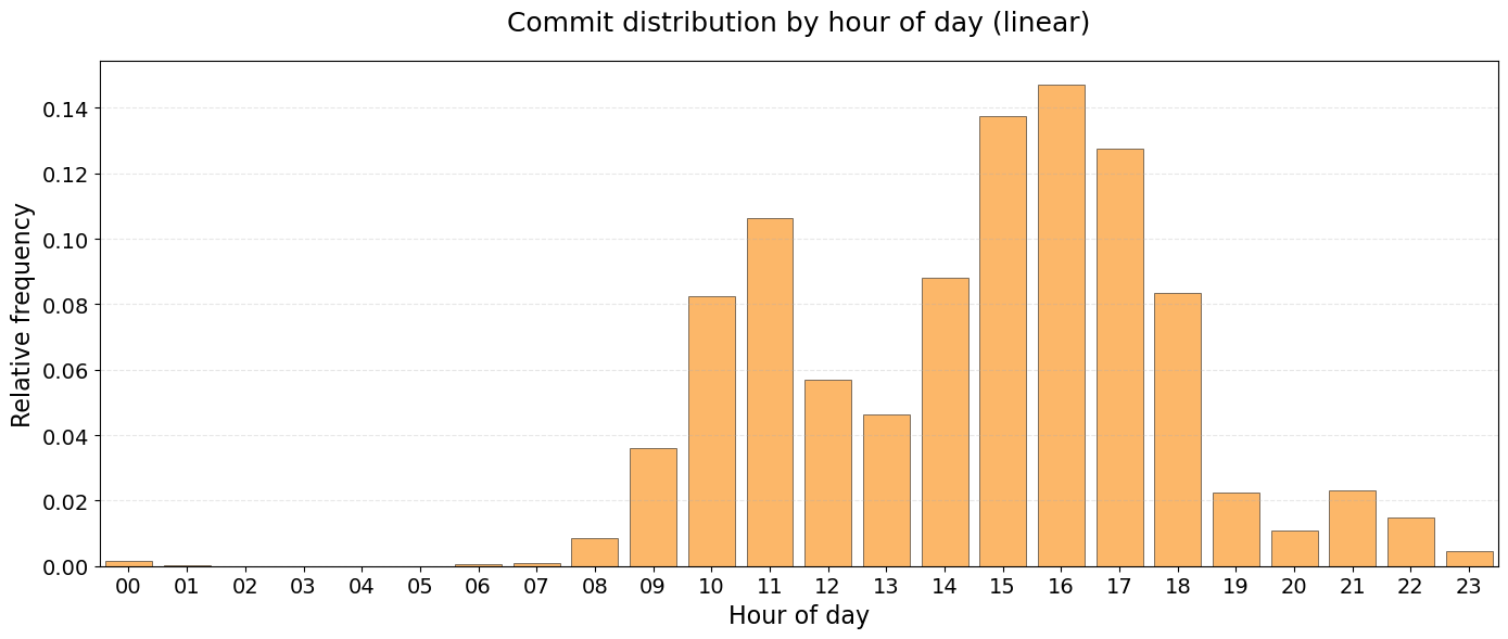
Hourly Distribution (Linear)
The next figure displays commit frequency across a 24-hour period.
fig, ax = plt.subplots(figsize=(14, 6))
ax.bar(
    hour_df.index,
    hour_df["distrib"],
    color=color,
    alpha=0.7,
    edgecolor="black",
    linewidth=0.5,
)
ax.set_title("Commit distribution by hour of day (linear)", fontsize=18, pad=20)
ax.set_xlabel("Hour of day", fontsize=16)
ax.set_ylabel("Relative frequency", fontsize=16)
ax.set_xlim(-0.5, 23.5)
ax.grid(axis="y", linestyle="--", alpha=0.3)
ax.set_xticks(range(24))
ax.set_xticklabels([f"{h:02d}" for h in range(24)])
plt.tick_params(axis="both", labelsize=14)
plt.tight_layout()
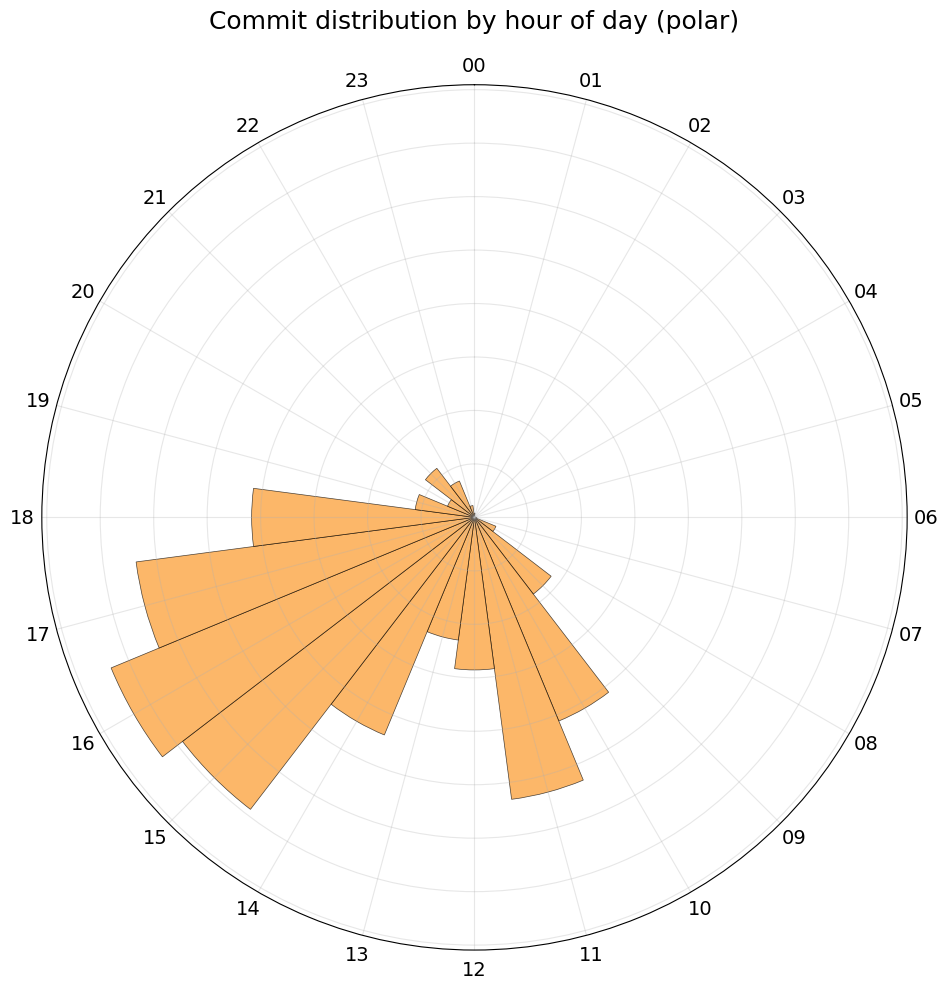
Hourly Distribution (polar)
This is the same data as avove, but plotted in polar coordinates.
fig, ax = plt.subplots(figsize=(10, 10), subplot_kw=dict(projection="polar"))
theta = np.linspace(0, 2 * np.pi, 24, endpoint=False)
radii = hour_df["distrib"].values
ax.bar(
    theta,
    radii,
    width=2 * np.pi / 24,
    color=color,
    alpha=0.7,
    edgecolor="black",
    linewidth=0.5,
)
ax.set_theta_zero_location("N")
ax.set_theta_direction(-1)
ax.set_thetagrids(range(0, 360, 15), [f"{h:02d}" for h in range(0, 24, 1)])
ax.set_ylim(0, max(radii) * 1.1)
ax.set_yticklabels([])
plt.tick_params(axis="both", labelsize=14)
ax.set_title("Commit distribution by hour of day (polar)", fontsize=18, pad=20)
ax.grid(True, alpha=0.3)
plt.tight_layout()
Temporal heatmap
The figure here is a two-dimensional heatmap correlating weekday and hour-of-day commit patterns. Data is normalized to show percentage of total commits.
commit_data = []
for i, (hour, weekday) in enumerate(zip(all_hours, all_weekdays)):
    commit_data.append({"hour": hour, "weekday": weekday})

commit_df = pd.DataFrame(commit_data)
heatmap_data = commit_df.groupby(["weekday", "hour"]).size().unstack(fill_value=0)
heatmap_data = heatmap_data.reindex(days_order)

all_hours_cols = list(range(24))
heatmap_data = heatmap_data.reindex(columns=all_hours_cols, fill_value=0)
heatmap_normalized = heatmap_data / heatmap_data.sum().sum() * 100
heatmap_normalized.head(3)
| hour | 0 | 1 | ... | 22 | 23 |
|---|---|---|---|---|---|
| weekday | |||||
| Monday | 0.000000 | 0.0 | ... | 0.499671 | 0.092045 |
| Tuesday | 0.039448 | 0.0 | ... | 0.197239 | 0.078895 |
| Wednesday | 0.078895 | 0.0 | ... | 0.262985 | 0.026298 |
3 rows × 24 columns
assert np.isclose(
    np.float64(heatmap_normalized.sum().sum()), 100.0, rtol=1e-10, atol=1e-10
)
fig, ax = plt.subplots(figsize=(16, 8))
im = ax.imshow(
    heatmap_normalized,
    aspect="auto",
    cmap="tol.YlOrBr",
    interpolation="nearest",
    vmin=0,
)
ax.set_xticks(np.arange(24))
ax.set_yticks(np.arange(len(days_order)))
ax.set_xticklabels([f"{h:02d}" for h in range(24)])
ax.set_yticklabels(days_order)
plt.setp(ax.get_xticklabels(), rotation=0, ha="center")
cbar = plt.colorbar(im, ax=ax)
cbar.set_label(
    "Percentage of total commits (%)", rotation=270, labelpad=20, fontsize=16
)
cbar.ax.tick_params(labelsize=14)
ax.set_title("Commit activity heatmap by hour and weekday", fontsize=18, pad=20)
ax.set_xlabel("Hour of day", fontsize=16)
ax.set_ylabel("Day of week", fontsize=16)
ax.set_xticks(np.arange(24) - 0.5, minor=True)
ax.set_yticks(np.arange(len(days_order)) - 0.5, minor=True)
plt.tick_params(axis="both", labelsize=14)
ax.grid(which="minor", color="gray", linestyle="-", linewidth=0.5, alpha=0.3)
plt.tight_layout()
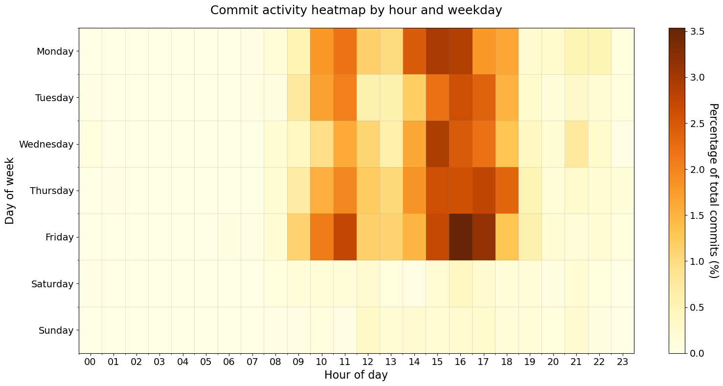
So it seems that friday 4 pm is my most productive hour of the week!