GPU Analytics Ep 3, Apply a function to the rows of a dataframe
The goal of this post is to compare the execution time between Pandas (CPU) and RAPIDS (GPU) dataframes, when applying a simple mathematical function to the rows of a dataframe.
Since the row-wise applied function is a re-projection of geographical cooordinates (WGS84 to Web Mercator), we are also going to compare the different methods with an equivalent native method of GeoPandas.
The present post is related to another post, in which I compared different ways to loop over Pandas dataframes.
Although I already had an environment running on AWS with RAPIDS cuDF (GPU dataframes) and the other GPU-related libraries ready (see the last post), I got into trouble when updating cuDF (from 0.6 to 0.7), pymapd and some other packages. Because these tools are fairly recent, you get some new releases very frequently! Anyway, I probably did something wrong… But I did not want to waste some time trying to fix this AWS instance. We are going to run the code on two different hardware environments:
- my laptop
- Google Collab
My laptop’s GPU is rather weak, and this is why we will switch to Collab in the second part of this post.
Pandas, GeoPandas and RAPIDS on my laptop
My laptop’s technical features:
- CPU: Intel i7-7700HQ @ 2.80GHz with 8 cores and 16GB of RAM
- GPU: NVIDIA GEFORCE GTX 1050Ti (Pascal architecture) with 4GB of RAM
The Python and package versions are the following ones:
%watermark
2019-05-21T13:39:09+02:00

CPython 3.7.3
IPython 7.5.0

compiler   : GCC 7.3.0
system     : Linux
release    : 4.15.0-50-generic
machine    : x86_64
processor  : x86_64
CPU cores  : 8
interpreter: 64bit
%watermark --iversions
geopandas  0.5.0
pandas     0.24.2
cudf       0.7.2+0.g3ebd286.dirty
numpy      1.16.3
numba      0.43.1
matplotlib 3.0.3
contextily 0.99.0.dev
Note the name of the cuDF version tag! :)
Data creation
First we create some artificial data: we generate n point coordinates within a given bounding box of Lyon, France. These coordinates corresponds to the longitude and latitude of the points, expressed in the World Geodetic System (WGS84).
def create_df(n=10000, lon_min=4.771813, lon_max=4.898377, lat_min=45.707367, lat_max=45.808263, seed=123):
    np.random.seed(seed)
    coords = np.random.rand(n, 2)
    coords[:,0] *= lon_max - lon_min
    coords[:,0] += lon_min
    coords[:,1] *= lat_max - lat_min
    coords[:,1] += lat_min
    return pd.DataFrame(data={
        'lon': coords[:,0],
        'lat': coords[:,1]})
df = create_df()
df.head(2)
| lon | lat | |
|---|---|---|
| 0 | 4.859961 | 45.736237 |
| 1 | 4.800524 | 45.762992 |
The row-wise user defined function : re-projecting the coordinates
From GeoPandas’ documentation:
Re-projecting is the process of changing the representation of locations from one coordinate system to another. All projections of locations on the Earth into a two-dimensional plane are distortions, the projection that is best for your application may be different from the projection associated with the data you import.
In our present use case, we are going to change the Coordinates Reference System (CRS) from WGS84 (also called EPSG4326) to Web Mercator (also called EPSG3857), often used in web mapping applications.
The Reference solution
In order to make sure that our User-Defined Function (UDF) is accurate and to have a reference solution, we are first going to perform this re-projection task with GeoPandas, which is an incredibly useful library when dealing with geospatial data. First we create a GeoDataFrame with our point coordinates:
crs = {'init': 'epsg:4326'}
gdf = gpd.GeoDataFrame(df.drop(['lat', 'lon'], axis=1), crs=crs, geometry=gpd.points_from_xy(df.lon, df.lat))
gdf.head(2)
| geometry | |
|---|---|
| 0 | POINT (4.859960926006008 45.73623731433915) |
| 1 | POINT (4.8005242273689 45.76299245494138) |
As you can see, the longitude and latitude coordinates got transformed into Shapely Point objects when creating the GeoDataFrame. Now we can change the coordinates referential system:
gdf = gdf.to_crs(epsg='3857')
gdf.head(2)
| geometry | |
|---|---|
| 0 | POINT (541008.3755581942 5738181.345632877) |
| 1 | POINT (534391.9125314779 5742449.601410745) |
Since we converted the CRS to Web Mercator, we can now plot the points on a map with background tiles provided by Stamen Design. We add these tiles using the contextily package.The following add_basemap function is taken from the GeoPandas documentation.
def add_basemap(ax, zoom, url='http://tile.stamen.com/terrain-background/tileZ/tileX/tileY.png'):
    xmin, xmax, ymin, ymax = ax.axis()
    basemap, extent = ctx.bounds2img(xmin, ymin, xmax, ymax, zoom=zoom, url=url)
    ax.imshow(basemap, extent=extent, interpolation='bilinear')
    ax.axis((xmin, xmax, ymin, ymax)) # restore original x/y limits

ax = gdf.plot(figsize=(12,12), markersize=5, color='k', alpha=0.2);
add_basemap(ax, zoom=12);
plt.axis('off');
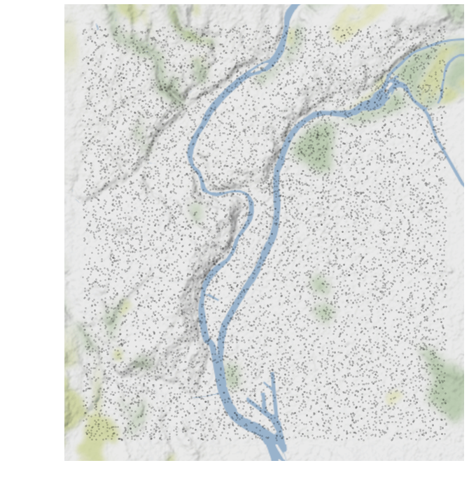
Of course, in the present case, this is not so usefull to visualize some random points on a map. At least we can check visually that they are in the bounding box…
The re-projection function
The formulae for the re-projection from EPSG4326 (WGS84) to EPSG3854 (Web Mercator) is taken from a pdf found on the web and entitled “Implementation Practice Web Mercator Map Projection”. It is a fairly simple one compared with other re-projections.
The first function to_EPSG3857_2 has two arguments: lon and lat, while the second one to_EPSG3857_4 has four. The second one is a non-value returning function, modifying the input arguments. Also, in order to be compatible with numba, I had to use the math library instead of numpy for the log and tan functions (from what I understand, the math module has been implemented in Numba, but some numpy functions do not have an implementation that can be inlined by Numba??).
def to_EPSG3857_2(lon, lat):
    a = 6378137.0
    return a * np.pi * lon / 180.0, a * np.log(np.tan(np.pi * (0.25 + lat / 360.0)))

def to_EPSG3857_4(lon, lat, x, y):
    a = 6378137.0
    n = lon.shape[0]
    for i in range(n):
        x[i] = a * np.pi * lon[i] / 180.0
        y[i] = a * math.log(math.tan(np.pi * (0.25 + lat[i] / 360.0)))
Let’s create 3 other functions:
to_EPSG3857_vectvectorized withnumpy(single thread)to_EPSG3857_numbaoptimized withnumba jit(single thread)to_EPSG3857_paraoptimized withnumba njit(explicit parallel loops, multi-threaded)
to_EPSG3857_vect = np.vectorize(to_EPSG3857_2)

to_EPSG3857_numba = jit(to_EPSG3857_4, nopython=True)

@njit(parallel=True)
def to_EPSG3857_para(lon, lat, x, y):
    a = 6378137.0
    n = lon.shape[0]
    for i in prange(n):
        x[i] = a * np.pi * lon[i] / 180.0
        y[i] = a * math.log(math.tan(np.pi * (0.25 + lat[i] / 360.0)))
A comparison of all the approaches
Let’s introduce a Timer helper class used later to collect all the timings (taken from a RAPIDS notebook):
class Timer(object):
    def __init__(self):
        self._timer = default_timer

    def __enter__(self):
        self.start()
        return self

    def __exit__(self, *args):
        self.stop()

    def start(self):
        """Start the timer."""
        self.start = self._timer()

    def stop(self):
        """Stop the timer. Calculate the interval in seconds."""
        self.end = self._timer()
        self.interval = self.end - self.start
And a function comparing all the approaches:
def compare(n=10000, tol=1.e-12, check=True, vect=True):

    time = {}
    time['n'] = n

    # 1 - create a Pandas dataframe
    timer = Timer(); timer.start()
    df = create_df(n)
    timer.stop(); time['1_create_df'] = timer.interval;

    if check:
        # 2 - convert the dataframe into a geodataframe
        timer = Timer(); timer.start()
        crs = {'init': 'epsg:4326'}
        geodf = gpd.GeoDataFrame(df.drop(['lat', 'lon'], axis=1), crs=crs, geometry=gpd.points_from_xy(df.lon, df.lat))
        timer.stop(); time['2_df_to_gdf'] = timer.interval

        # 3 - convert the CRS using GeoPandas to_crs() method
        timer = Timer(); timer.start()
        geodf = geodf.to_crs(epsg='3857')
        timer.stop(); time['3_gdf_to_crs'] = timer.interval

    if vect:
        # 4 - convert the CRS using vfunc
        timer = Timer(); timer.start()
        xp, yp = to_EPSG3857_vect(df.lon.values, df.lat.values)
        timer.stop(); time['4_np_vectorize'] = timer.interval

        if check:
            # access the transformed coordinates of the geodataframe
            x_ref = geodf.geometry.x.values
            y_ref = geodf.geometry.y.values

            # check the results of np.vectorize as compared to geopandas to_crs
            assert np.linalg.norm(xp-x_ref) / np.linalg.norm(x_ref) < tol
            assert np.linalg.norm(yp-y_ref) / np.linalg.norm(y_ref) < tol
        del xp, yp

    # 5 - convert the CRS using Numba
    df['x'] = 0.
    df['y'] = 0.
    timer = Timer(); timer.start()
    to_EPSG3857_numba(df.lon.values, df.lat.values, df.x.values, df.y.values)
    timer.stop(); time['5_numba'] = timer.interval

    if check:
        # access the transformed coordinates values
        x_1 = df.x.values
        y_1 = df.y.values

        # check the results of np.vectorize as compared to geopandas to_crs
        assert np.linalg.norm(x_1-x_ref) / np.linalg.norm(x_ref) < tol
        assert np.linalg.norm(y_1-y_ref) / np.linalg.norm(y_ref) < tol
        df.drop(['x', 'y'], axis=1, inplace=True)

    # 6 - convert the CRS using Numba parallel
    df['x'] = 0.
    df['y'] = 0.
    timer = Timer(); timer.start()
    to_EPSG3857_para(df.lon.values, df.lat.values, df.x.values, df.y.values)
    timer.stop(); time['6_numba_para'] = timer.interval

    if check:
        # access the transformed coordinates values
        x_1 = df.x.values
        y_1 = df.y.values

        # check the results of np.vectorize as compared to geopandas to_crs
        assert np.linalg.norm(x_1-x_ref) / np.linalg.norm(x_ref) < tol
        assert np.linalg.norm(y_1-y_ref) / np.linalg.norm(y_ref) < tol
    df.drop(['x', 'y'], axis=1, inplace=True)

    # 7 - create a GPU dataframe from the Pandas dataframe
    timer = Timer(); timer.start()
    gpudf = cudf.DataFrame.from_pandas(df)
    timer.stop(); time['7_cudf_from_df'] = timer.interval

    # 8 - convert the CRS on the GPU using apply_rows and to_EPSG3857_4
    timer = Timer(); timer.start()
    gpudf = gpudf.apply_rows(
        to_EPSG3857_4,
        incols=['lon', 'lat'],
        outcols=dict(x=np.float64, y=np.float64),
        kwargs=dict())
    timer.stop(); time['8_cudf_apply_rows'] = timer.interval

    if check:
        # 9 - convert the cudf to a Pandas dataframe
        timer = Timer(); timer.start()
        df_2 = gpudf[['x', 'y']].to_pandas()
        timer.stop(); time['9_cudf_to_df'] = timer.interval

        # access the transformed coordinates values
        x_2 = df_2.x.values
        y_2 = df_2.y.values

        # check the results of to_EPSG3857_4 as compared to geopandas to_crs
        assert np.linalg.norm(x_2-x_ref) / np.linalg.norm(x_ref) < tol
        assert np.linalg.norm(y_2-y_ref) / np.linalg.norm(y_ref) < tol

        del df_2

    del df, gpudf
    gc.collect()

    return time
Now we loop on different array sizes. For each size we run 3 trials and only keep the smallest elapsed time:
res = []
for i in range(1,6):
    n = 10**i
    for j in range(3):
        d = compare(n)
        d['trial'] = j
        res.append(d)
res = pd.DataFrame(res)
res = res.groupby('n').min()
res.drop('trial', axis=1, inplace=True)
We are going to plot these results on two different firgures: the first one is about the dataframe and geodataframe creation, the second one about the different re-projecting methods.
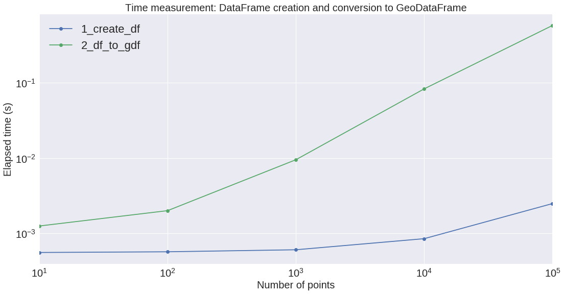
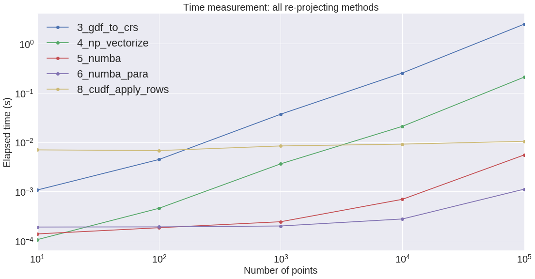
We can see that the conversion from Pandas to GeoPandas is rather expensive. Also, regarding the re-projection, GeoPandas is by far the slowest. GeoPandas is using the pyproj library (which is probably using a sequential Python loop on the Shapely objects??).
Regarding the re-projection process, Numba on the CPU seems to be the most efficient implementation on the small/medium size arrays.
Well now that we validated the approach by comparing the UDF results with GeoPandas transformed coordinates, we are going to create a smaller function without all the assertions of the above function. This allows us to skip the GeoPandas part, which is taking too long when the number of points is above a million. And we are going to run it on Google Colab.
Reduced comparison on Google Colab
Now let us run the apply row functions on Google Colab. This section is inspired by this post: Run RAPIDS on Google Colab — For Free. Basically you just need to copy the notebook file to your Google drive since we are generating all the data within the notebook.
First we make sure to use a graphics processing unit by setting Edit > Notebook settings > Hardware accelerator to GPU. We can see that the available GPU is actually a recent one: Tesla T4 (Turing) with 15GB of memory:
!nvidia-smi
Wed Jun 12 14:22:55 2019
+-----------------------------------------------------------------------------+
| NVIDIA-SMI 418.67       Driver Version: 410.79       CUDA Version: 10.0     |
|-------------------------------+----------------------+----------------------+
| GPU  Name        Persistence-M| Bus-Id        Disp.A | Volatile Uncorr. ECC |
| Fan  Temp  Perf  Pwr:Usage/Cap|         Memory-Usage | GPU-Util  Compute M. |
|===============================+======================+======================|
|   0  Tesla T4            Off  | 00000000:00:04.0 Off |                    0 |
| N/A   71C    P0    30W /  70W |      0MiB / 15079MiB |      0%      Default |
+-------------------------------+----------------------+----------------------+

+-----------------------------------------------------------------------------+
| Processes:                                                       GPU Memory |
|  GPU       PID   Type   Process name                             Usage      |
|=============================================================================|
|  No running processes found                                                 |
+-----------------------------------------------------------------------------+
However, note that sometimes we get a K80 instead of T4 GPU instance. Then you need to reset it until you get a T4 (Runtime > Reset all runtimes). Also, the CPU is a dual core Intel Xeon @ 2.20GHz (12 GB RAM).
Now we are going to install miniconda and the other required packages:
# intall miniconda
!wget -c https://repo.continuum.io/miniconda/Miniconda3-4.5.4-Linux-x86_64.sh
!chmod +x Miniconda3-4.5.4-Linux-x86_64.sh
!bash ./Miniconda3-4.5.4-Linux-x86_64.sh -b -f -p /usr/local

# install RAPIDS packages
!conda install -q -y --prefix /usr/local -c conda-forge \
  -c rapidsai-nightly/label/cuda10.0 -c nvidia/label/cuda10.0 \
  cudf cuml

# set environment vars
import sys, os, shutil
sys.path.append('/usr/local/lib/python3.6/site-packages/')
os.environ['NUMBAPRO_NVVM'] = '/usr/local/cuda/nvvm/lib64/libnvvm.so'
os.environ['NUMBAPRO_LIBDEVICE'] = '/usr/local/cuda/nvvm/libdevice/'

# copy .so files to current working dir
for fn in ['libcudf.so', 'librmm.so']:
  shutil.copy('/usr/local/lib/'+fn, os.getcwd())
!conda install -y -c conda-forge watermark
%watermark
2019-06-12T14:29:30+00:00

CPython 3.6.7
IPython 5.5.0

compiler   : GCC 8.2.0
system     : Linux
release    : 4.14.79+
machine    : x86_64
processor  : x86_64
CPU cores  : 2
interpreter: 64bit
%watermark --iversions
numba      0.40.1
numpy      1.16.4
cudf       0.8.0a1+701.gbeac92b.dirty
matplotlib 3.0.3
IPython    5.5.0
pandas     0.24.2
Still a “dirty” cuDF realease :)
A reduced comparison
This time the reduced compare function only has the following steps (we keep the step numbers from the previous section):
- 1 - create a Pandas dataframe
- 5 - convert the CRS using Numba
- 6 - convert the CRS using Numba parallel
- 7 - create a GPU dataframe from the Pandas dataframe
- 8 - convert the CRS on the GPU using apply_rows and to_EPSG3857_4
Here are the results:
| 1_create_df | 5_numba | 6_numba_para | 7_cudf_from_df | 8_cudf_apply_rows | |
|---|---|---|---|---|---|
| n | |||||
| 10 | 0.000496 | 0.000228 | 0.000197 | 0.004118 | 0.004346 |
| 100 | 0.000460 | 0.000223 | 0.000195 | 0.003854 | 0.004443 |
| 1_000 | 0.000546 | 0.000288 | 0.000289 | 0.005034 | 0.006692 |
| 10_000 | 0.000749 | 0.000866 | 0.000651 | 0.006025 | 0.007745 |
| 100_000 | 0.003069 | 0.006858 | 0.004497 | 0.007383 | 0.009915 |
| 1_000_000 | 0.026337 | 0.067422 | 0.043061 | 0.019195 | 0.023371 |
| 10_000_000 | 0.296810 | 0.622501 | 0.398296 | 0.120603 | 0.148041 |
| 100_000_000 | 3.047611 | 6.232928 | 3.996533 | 1.125418 | 1.045445 |
On the next figure, we can see the benefit of using cuDFs when dealing with arrays larger than a million. It seems that the cuDF slope is increasing a little bit slower that the CPU Numba ones. However, the CPU is not so powerful: it would be interesting to perform a measurment on a faster CPU with many cores.
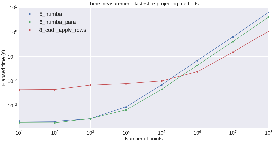
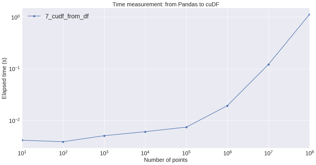
Also we measured the cost of moving data from the motherboard to the GPU device:
Conclusion:
- RAPIDS cuDF ìs very efficient when dealing with large arrays and row-wise operations
- Numba
njitis also efficient while very easy to use, and for any size of array - Google Colab make it easy to test different hardware options