Create a routable pedestrian network with elevation
In this blog post, we will explore how to create a routable pedestrian network with elevation using Python and OSMnx. OSMnx is a Python library that allows you to retrieve OpenStreetMap (OSM) data and work with street networks, among other things.
Here’s a summary of the steps followed in the blog post:
- Graph download with OSMnx
- Graph simplification with Pandas
- Network visualization
- Incorporating elevation data into nodes
- Computing edge walking time attribute
- Save the edges and nodes to files
As the underlying motivation for this graph processing steps, our aim is to run path algorithms on this pedestrian network.
System and package versions
We are operating on Python version 3.11.7 and running on a Linux x86_64 machine.
contextily             : 1.5.0
fiona                  : 1.9.5
geopandas              : 0.14.1
matplotlib             : 3.8.2
numpy                  : 1.26.3
osmnx                  : 1.8.1
pandas                 : 2.1.4
rasterio               : 1.3.9
shapely                : 2.0.2
Imports
import contextily as cx
import matplotlib.pyplot as plt
import numpy as np
import osmnx as ox
import pandas as pd
import rasterio as rio
from shapely.geometry import LineString, Point

DTP_FP = "./lyon_dem.tif"
OUTPUT_NODES_FP = "./nodes_lyon_pedestrian_network.GeoJSON"
OUTPUT_EDGES_FP = "./edges_lyon_pedestrian_network.GeoJSON"
The file paths for Digital Terrain Model (DTM), and the output nodes and edges GeoJSON files are defined just above.
Graph download with OSMnx
We begin by defining a bounding box using the coordinates in EPSG:4326 (WGS 84). This box encapsulates the geographical area of interest:
bbox = (4.5931155, 45.515971, 5.0473875, 45.970243)
Now, let’s utilize the ox.graph_from_bbox function with specific parameters, besides the bounding box:
network_type (string {"all_private", "all", "bike", "drive", "drive_service", "walk"}): what type of street network to getsimplify (bool): If set toTrue, the graph topology is simplified using thesimplify_graphfunction.retain_all (bool): WhenTrue, the function returns the entire graph even if it’s not fully connected. Otherwise, it retains only the largest weakly connected component.truncate_by_edge (bool): Enabling this option retains nodes outside the bounding box if at least one of a node’s neighbors is within the bounding box.
%%time
G = ox.graph_from_bbox(
    north=bbox[3],
    south=bbox[1],
    east=bbox[0],
    west=bbox[2],
    network_type="walk",
    simplify=True,
    retain_all=True,
    truncate_by_edge=True,
)
CPU times: user 52.5 s, sys: 1.19 s, total: 53.7 s
Wall time: 59.3 s
The output graph is a NetworkX object. We can explore some of the graph properties, such as whether it is directed:
G.is_directed()
True
Now we convert the graph into GeoDataFrames for nodes and edges, respectively:
%%time
nodes_gdf, edges_gdf = ox.graph_to_gdfs(G)
CPU times: user 7.92 s, sys: 85.7 ms, total: 8.01 s
Wall time: 8.02 s
Let’s have a look at the Coordinate Reference System (CRS):
nodes_gdf.crs
<Geographic 2D CRS: EPSG:4326>
Name: WGS 84
Axis Info [ellipsoidal]:
- Lat[north]: Geodetic latitude (degree)
- Lon[east]: Geodetic longitude (degree)
Area of Use:
- name: World.
- bounds: (-180.0, -90.0, 180.0, 90.0)
Datum: World Geodetic System 1984 ensemble
- Ellipsoid: WGS 84
- Prime Meridian: Greenwich
The GeoDataFrames have many columns that we won’t use:
nodes_gdf.columns
Index(['y', 'x', 'street_count', 'highway', 'ref', 'geometry'], dtype='object')
edges_gdf.columns
Index(['osmid', 'highway', 'oneway', 'reversed', 'length', 'geometry', 'lanes',
       'ref', 'maxspeed', 'bridge', 'name', 'service', 'width', 'junction',
       'access', 'tunnel', 'est_width', 'area'],
      dtype='object')
In the next section, we will process the graph, removing many useless features for our pedestrian routing use-case.
Graph simplification with Pandas
Highway type
We initiate the process by excluding major roads, deemed less pedestrian-friendly based on data checked on openstreetmap.org:
edges_gdf = edges_gdf.loc[edges_gdf.highway != "trunk"]
edges_gdf = edges_gdf.loc[edges_gdf.highway != "trunk_link"]
Let’s have a look at the various highway types remaining within our network. The service type is the most prevalent, followed by residential and footway:
edges_gdf["highway"].value_counts()[:20]
highway
service                   98658
residential               85920
footway                   82620
unclassified              46060
tertiary                  26462
path                      25706
track                     21636
secondary                 19220
primary                   13192
corridor                   4778
[footway, steps]           3718
living_street              3316
pedestrian                 2850
steps                      2074
[footway, service]         1376
[footway, residential]     1108
[track, residential]        978
[track, path]               884
[residential, path]         614
[residential, service]      476
Name: count, dtype: int64
Edge column selection and renaming
# edge column selection and renaming
edges = edges_gdf[["geometry"]].reset_index(drop=False)
edges = edges.rename(columns={"u": "tail", "v": "head"})
edges.drop("key", axis=1, inplace=True)
edges.head(3)
| tail | head | geometry | |
|---|---|---|---|
| 0 | 143196 | 387462616 | LINESTRING (5.02801 45.67790, 5.02769 45.67791... |
| 1 | 143403 | 21714981 | LINESTRING (4.87754 45.73383, 4.87739 45.73379) |
| 2 | 143403 | 9226919131 | LINESTRING (4.87754 45.73383, 4.87723 45.73393) |
Make sure we get each edge in both directions
This step ensures that each edge is represented in both directions (tail to head and head to tail).
# we select one direction between each pair couples
edges["min_vert"] = edges[["tail", "head"]].min(axis=1)
edges["max_vert"] = edges[["tail", "head"]].max(axis=1)
Compute length in a projected CRS:
edges = edges.to_crs("EPSG:2154")
edges["length"] = edges.geometry.map(lambda g: g.length)
edges = edges.to_crs("EPSG:4326")
Sort the edges based on minimum vertex, maximum vertex, and length, then remove parallel edges, keeping only the shortest one.
edges = edges.sort_values(by=["min_vert", "max_vert", "length"], ascending=True)
edges = edges.drop_duplicates(subset=["min_vert", "max_vert"], keep="first")
edges = edges.drop(["min_vert", "max_vert"], axis=1)
We reverse the edges and concatenate them with the original edges to ensure representation in both directions.
edges_reverse = edges.copy(deep=True)
edges_reverse[["tail", "head"]] = edges_reverse[["head", "tail"]]
edges_reverse.geometry = edges_reverse.geometry.map(lambda g: g.reverse())
edges = pd.concat((edges, edges_reverse), axis=0)
We remove loops, then reset the index.
edges = edges.sort_values(by=["tail", "head"])
edges = edges.loc[edges["tail"] != edges["head"]]
edges.reset_index(drop=True, inplace=True)
edges.shape
(440248, 4)
Node column selection
nodes = nodes_gdf[["geometry"]].copy(deep=True)
nodes = nodes.reset_index(drop=False)
nodes.head(3)
| osmid | geometry | |
|---|---|---|
| 0 | 126096 | POINT (4.78386 45.78928) |
| 1 | 143196 | POINT (5.02801 45.67790) |
| 2 | 143356 | POINT (4.84325 45.71446) |
Node reindexing
The following function reindexes node IDs contiguously and updates both the nodes and edges DataFrames:
def reindex_nodes(
    nodes, edges, node_id_col="osmid", tail_id_col="tail", head_id_col="head"
):
    if node_id_col == "id":
        node_id_col = "id_old"
        nodes = nodes.rename(columns={"id": node_id_col})

    assert "geometry" in nodes

    # reindex the nodes and update the edges
    nodes = nodes.reset_index(drop=True)
    if "id" in nodes.columns:
        nodes = nodes.drop("id", axis=1)
    nodes["id"] = nodes.index
    edges = pd.merge(
        edges,
        nodes[["id", node_id_col]],
        left_on=tail_id_col,
        right_on=node_id_col,
        how="left",
    )
    edges.drop([tail_id_col, node_id_col], axis=1, inplace=True)
    edges.rename(columns={"id": tail_id_col}, inplace=True)
    edges = pd.merge(
        edges,
        nodes[["id", node_id_col]],
        left_on=head_id_col,
        right_on=node_id_col,
        how="left",
    )
    edges.drop([head_id_col, node_id_col], axis=1, inplace=True)
    edges.rename(columns={"id": head_id_col}, inplace=True)

    # reorder the columns to have tail and head node vertices first
    cols = edges.columns
    extra_cols = [c for c in cols if c not in ["tail", "head"]]
    cols = ["tail", "head"] + extra_cols
    edges = edges[cols]

    # cleanup
    if node_id_col in nodes:
        nodes = nodes.drop(node_id_col, axis=1)

    return nodes, edges


nodes, edges = reindex_nodes(
    nodes, edges, node_id_col="osmid", tail_id_col="tail", head_id_col="head"
)
edges.head(3)
| tail | head | geometry | length | |
|---|---|---|---|---|
| 0 | 1 | 14988 | LINESTRING (5.02801 45.67790, 5.02769 45.67791... | 158.045057 |
| 1 | 5 | 714 | LINESTRING (4.87754 45.73383, 4.87739 45.73379) | 12.138616 |
| 2 | 5 | 140378 | LINESTRING (4.87754 45.73383, 4.87761 45.73387... | 11.072676 |
edges.shape
(440248, 4)
nodes.set_index("id", inplace=True)
nodes.head(3)
| geometry | |
|---|---|
| id | |
| 0 | POINT (4.78386 45.78928) |
| 1 | POINT (5.02801 45.67790) |
| 2 | POINT (4.84325 45.71446) |
nodes.shape
(167128, 1)
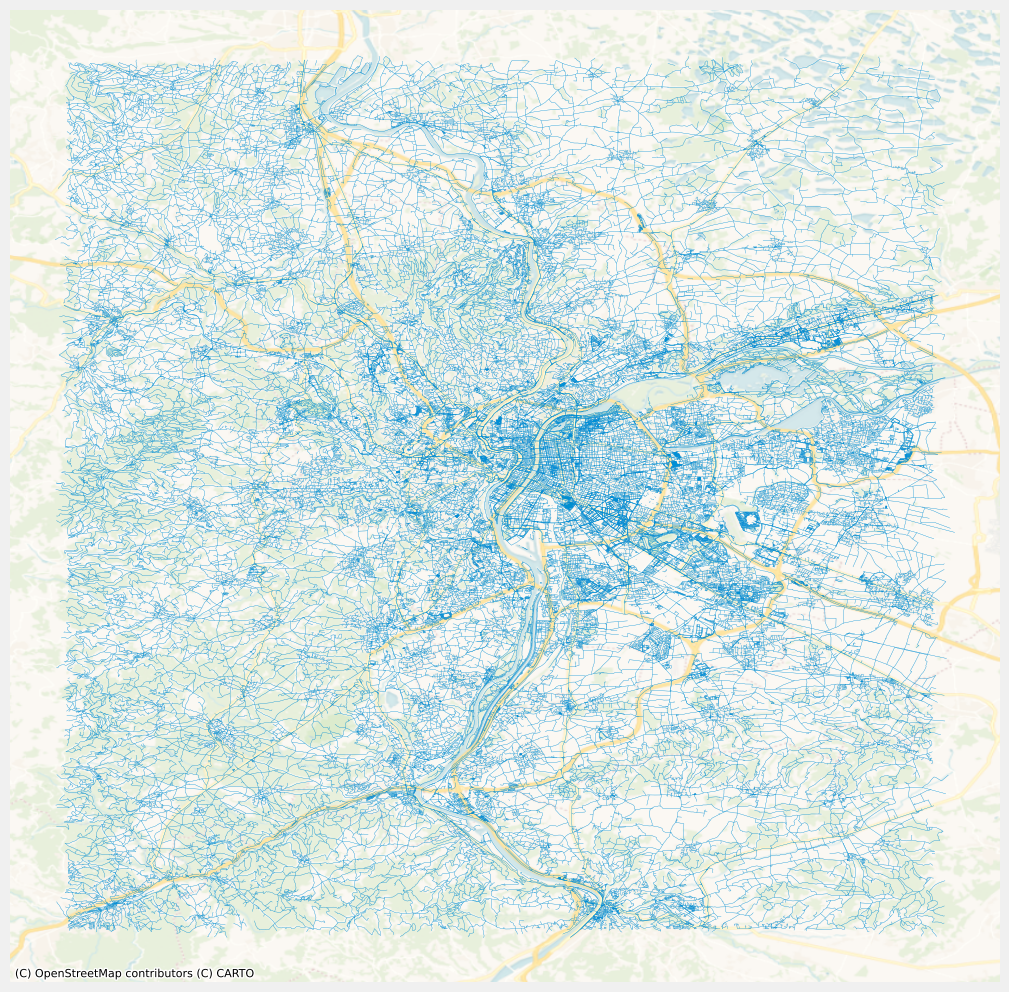
Network visualization
ax = edges.plot(linewidth=0.2, alpha=0.7, figsize=(12, 12))
cx.add_basemap(
    ax, source=cx.providers.CartoDB.VoyagerNoLabels, crs=edges.crs.to_string()
)
_ = plt.axis("off")

Incorporating elevation data into nodes
The following piece of code transforms the node coordinates to Lambert 93 for compatibility with the elevation data source. After extracting latitude and longitude coordinates, it samples elevation data from a Digital Terrain Model (DTM) using the rasterio library. The DTM raster file comes from a previous post:
The resulting elevation values are added to the nodes DataFrame, with special consideration for handling invalid elevation values.
Note that it was also possible to add the elevation data with OSMnx, using osmnx.elevation.add_node_elevations_raster.
# extract point coordinates in Lambert 93
nodes = nodes.to_crs("EPSG:2154")
lon_lam93 = nodes.geometry.apply(lambda p: p.x)
lat_lam93 = nodes.geometry.apply(lambda p: p.y)
nodes = nodes.to_crs("EPSG:4326")
point_coords = list(zip(lon_lam93, lat_lam93))
dem = rio.open(DTP_FP)
%%time
nodes["z"] = [x[0] for x in dem.sample(point_coords)]
CPU times: user 2.36 s, sys: 232 ms, total: 2.59 s
Wall time: 2.6 s
nodes.loc[nodes["z"] <= -99999, "z"] = np.nan
nodes.head(3)
| geometry | z | |
|---|---|---|
| id | ||
| 0 | POINT (4.78386 45.78928) | 257.890015 |
| 1 | POINT (5.02801 45.67790) | 251.649994 |
| 2 | POINT (4.84325 45.71446) | 163.899994 |
Computing edge walking time attribute
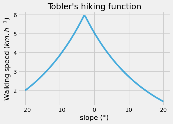
This section focuses on calculating the walking time attribute for each edge in the network. It begins by describing the simple Tobler’s hiking function, which estimates walking speed based on the slope of the terrain:
\[v = 6 e^{-3.5 \left| \tan(\theta) + 0.05 \right|}\]$v$ is the walking speed and $\theta$ the slope angle. Let’s plot this function:
def walking_speed_kmh(slope_deg):
    theta = np.pi * slope_deg / 180.0
    return 6.0 * np.exp(-3.5 * np.abs(np.tan(theta) + 0.05))

x = np.linspace(-20, 20, 100)
y = np.array(list(map(walking_speed_kmh, x)))

fig, ax = plt.subplots(figsize=(6, 4))
_ = plt.plot(x, y, alpha=0.7)
_ = ax.set(
    title="Tobler's hiking function",
    xlabel="slope (°)",
    ylabel="Walking speed ($km.h^{-1}$)",
)

To calculate the edge travel time, it is necessary to first compute the edge slope by utilizing the elevation information from the endpoints. We create some edge features, for the tail and head elevations:
edges = pd.merge(
    edges,
    nodes[["z"]].rename(columns={"z": "tail_z"}),
    left_on="tail",
    right_index=True,
    how="left",
)
edges = pd.merge(
    edges,
    nodes[["z"]].rename(columns={"z": "head_z"}),
    left_on="head",
    right_index=True,
    how="left",
)
In order to compute the slope angle, we are going to use the curvilinear length instead of the Euclidean distance between endpoints, considering the curvy nature of the linestrings.:
linestring = edges.iloc[0].geometry
linestring

This function, compute_slope, calculates the slope angle of a triangle based on its attributes. We start by making sure that the edge length is always strictly greater than zero:
edges["length"].min()
0.011105097809826743
def compute_slope(triangle_att):
    """
    triangle_att must be [tail_z, head_z, length]
    """
    tail_z, head_z, length = triangle_att

    x = (head_z - tail_z) / length
    theta = np.arctan(x)
    theta_deg = theta * 180.0 / np.pi

    # Limits the slope angle to a maximum of 20.0 degrees and
    # a minimum of -20.0 degrees
    theta_deg = np.amin([theta_deg, 20.0])
    theta_deg = np.amax([theta_deg, -20.0])

    return theta_deg
edges["slope_deg"] = edges[["tail_z", "head_z", "length"]].apply(
    compute_slope, raw=True, axis=1
)
Note that we could have computed slope_deg using Pandas column operations, and without applying a row function.
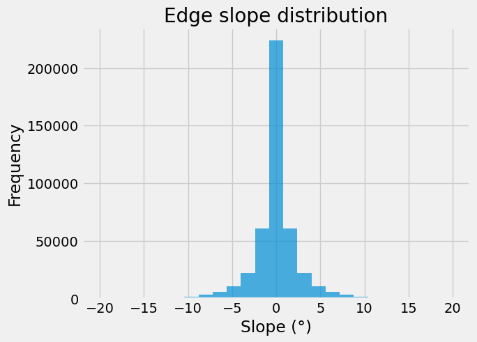
Here is the distribution of the linestrings’ slope over our network.
ax = edges.slope_deg.plot.hist(bins=25, alpha=0.7)
_ = ax.set(title="Edge slope distribution", xlabel="Slope (°)")

Now we can apply Tobler’s hiking function to each edge and compute the travel time:
edges["walking_speed_kmh"] = edges.slope_deg.map(lambda s: walking_speed_kmh(s))
edges["travel_time_s"] = 3600.0 * 1.0e-3 * edges["length"] / edges.walking_speed_kmh
# cleanup
edges.drop(
    ["tail_z", "head_z", "length", "length", "slope_deg", "walking_speed_kmh"],
    axis=1,
    inplace=True,
)
edges.head(3)
| tail | head | geometry | travel_time_s | |
|---|---|---|---|---|
| 0 | 1 | 14988 | LINESTRING (5.02801 45.67790, 5.02769 45.67791... | 108.644212 |
| 1 | 5 | 714 | LINESTRING (4.87754 45.73383, 4.87739 45.73379) | 8.478205 |
| 2 | 5 | 140378 | LINESTRING (4.87754 45.73383, 4.87761 45.73387... | 7.740962 |
Save the edges and nodes to files
Ultimately, we will save our network as two dataframes, one for nodes and one for edges. Below is the list of supported drivers for the output format:
fiona.supported_drivers
{'DXF': 'rw',
 'CSV': 'raw',
 'OpenFileGDB': 'raw',
 'ESRIJSON': 'r',
 'ESRI Shapefile': 'raw',
 'FlatGeobuf': 'raw',
 'GeoJSON': 'raw',
 'GeoJSONSeq': 'raw',
 'GPKG': 'raw',
 'GML': 'rw',
 'OGR_GMT': 'rw',
 'GPX': 'rw',
 'Idrisi': 'r',
 'MapInfo File': 'raw',
 'DGN': 'raw',
 'PCIDSK': 'raw',
 'OGR_PDS': 'r',
 'S57': 'r',
 'SQLite': 'raw',
 'TopoJSON': 'r'}
We are going to use the GeoJSON driver:
%%time
nodes.to_file(OUTPUT_NODES_FP, driver="GeoJSON", crs="EPSG:4326")
edges.to_file(OUTPUT_EDGES_FP, driver="GeoJSON", crs="EPSG:4326")
CPU times: user 21.7 s, sys: 124 ms, total: 21.8 s
Wall time: 21.9 s
!ls -l *.GeoJSON
-rw-rw-r-- 1 francois francois 127182433 Jan 30 18:28 edges_lyon_pedestrian_network.GeoJSON
-rw-rw-r-- 1 francois francois  25986369 Jan 30 18:27 nodes_lyon_pedestrian_network.GeoJSON