Calculating walking isochrones with Python
In this blog post, we’ll explore how to calculate walking isochrones using Python, taking into account the slope of the terrain. An isochrone is a line connecting all points that can be reached within a certain time from/to a specified location. By incorporating slope into our calculations, we can create more accurate isochrones.
We’ll use a pedestrian network dataset for Lyon, France, and demonstrate how to load the data, find the closest node to a point of interest, and calculate isochrones using Dijkstra’s algorithm.
Imports
import contextily as cx
import geopandas as gpd
import matplotlib.pyplot as plt
import numpy as np
import pandas as pd
import pyproj
import xyzservices.providers as xyz
from edsger.path import Dijkstra
from shapely import concave_hull
from shapely.geometry import MultiPoint, Point
from shapely.ops import transform
from sklearn.neighbors import KDTree

INPUT_NODES_FP = "./nodes_lyon_pedestrian_network.GeoJSON"
INPUT_EDGES_FP = "./edges_lyon_pedestrian_network.GeoJSON"

FS = (8, 8)  # figure size
We are operating on Python version 3.11.7 and running on a Linux x86_64 machine.
contextily             : 1.5.0
geopandas              : 0.14.3
matplotlib             : 3.8.3
numpy                  : 1.26.4
pandas                 : 2.2.1
pyproj                 : 3.6.1
xyzservices            : 2023.10.1
edsger                 : 0.0.13
shapely                : 2.0.3
sklearn                : 1.4.1.post1
Load the network
In this section, we load the nodes and edges datasets from GeoJSON files. The edges dataset has a travel time that takes edge slope into account. This directed network was created in a previous post: Create a routable pedestrian network with elevation
%%time
nodes = gpd.read_file(INPUT_NODES_FP)
nodes = nodes.set_index("id")
nodes.head(3)
CPU times: user 6.58 s, sys: 13.3 ms, total: 6.59 s
Wall time: 6.64 s
| z | geometry | |
|---|---|---|
| id | ||
| 0 | 257.890015 | POINT (4.78386 45.78928) |
| 1 | 251.649994 | POINT (5.02801 45.67790) |
| 2 | 163.899994 | POINT (4.84325 45.71446) |
%%time
edges = gpd.read_file(INPUT_EDGES_FP, index=False)
edges = edges[["tail", "head", "travel_time_s"]]
edges.head(3)
CPU times: user 20.3 s, sys: 140 ms, total: 20.4 s
Wall time: 20.5 s
| tail | head | travel_time_s | |
|---|---|---|---|
| 0 | 1 | 14988 | 108.643949 |
| 1 | 5 | 714 | 8.478201 |
| 2 | 5 | 140378 | 7.740958 |
Find closest node from point of interest
In order to compute the isochrones, we first need to find the closest node to our Point Of Interest (POI). We’ve chosen a POI location in the center of the Croix-Rousse district in Lyon. This location is interesting because it’s a hilly area with a lot of variation in elevation, which will make for some interesting isochrones.

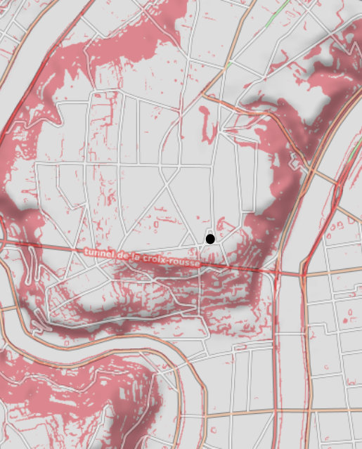
To better understand the terrain of our area of interest, here is a topographic map that displays the changes in elevation.

Note that the graph is not planar, which can be due to features such as a straight pedestrian tunnel under a hill. This means that the graph cannot be drawn in two dimensions without edges crossing each other. This can create challenges when generating the isochrones with concave hulls, as it may result in “weakly” connected sub-regions.
Here’s the code to define the POI and convert it to a projected coordinate reference system (Lambert 93) using the pyproj library.
x, y = 4.831721769832956, 45.774505209895295
poi_wgs84 = Point(x, y)

wgs84 = pyproj.CRS("EPSG:4326")
lam93 = pyproj.CRS("EPSG:2154")  # Lambert 93
project = pyproj.Transformer.from_crs(wgs84, lam93, always_xy=True).transform
poi_lam93 = transform(project, poi_wgs84)
Next we add new columns to the nodes dataset with the Lambert 93 coordinates and transform the dataset back to WGS84:
nodes = nodes.to_crs("EPSG:2154")
nodes["x_2154"] = nodes.geometry.x
nodes["y_2154"] = nodes.geometry.y
nodes = nodes.to_crs("EPSG:4326")
X = nodes[["x_2154", "y_2154"]].values
To find the closest node to the POI, we create a KDTree using the Lambert 93 coordinates of the nodes and query the tree for the n_connectors closest nodes to the POI. A KDTree is a data structure that allows for efficient search of nearest neighbors in two-dimensional spaces.
%%time
tree = KDTree(X)
CPU times: user 37.5 ms, sys: 0 ns, total: 37.5 ms
Wall time: 36.8 ms
x, y = poi_lam93.x, poi_lam93.y
%%time
n_connectors = 5
dist, ind = tree.query([[x, y]], k=n_connectors)
CPU times: user 218 µs, sys: 0 ns, total: 218 µs
Wall time: 208 µs
Here are the distances in meters to the n_connectors closest nodes:
dist
array([[12.43965184, 12.53458074, 16.07413804, 24.7330727 , 31.14538281]])
We can use these indices to select the closest nodes from the original nodes dataset:
ind
array([[ 32115, 109096, 109094, 13949, 135028]])
nodes.iloc[ind[0]]
| z | geometry | x_2154 | y_2154 | |
|---|---|---|---|---|
| id | ||||
| 32115 | 250.250000 | POINT (4.83156 45.77452) | 842318.103805 | 6.521085e+06 |
| 109096 | 250.240005 | POINT (4.83158 45.77456) | 842319.218654 | 6.521089e+06 |
| 109094 | 250.330002 | POINT (4.83154 45.77444) | 842316.539786 | 6.521075e+06 |
| 13949 | 250.460007 | POINT (4.83151 45.77434) | 842314.689130 | 6.521064e+06 |
| 135028 | 250.270004 | POINT (4.83211 45.77444) | 842360.907650 | 6.521077e+06 |
Create the connectors
Now that we have identified the n_connectors closest nodes to the POI, we need to create connectors between the POI and these nodes. These connectors will allow us to include the POI in our graph and compute the shortest path from the POI to any other node.
First, we create a new index for the POI by finding the maximum index in the nodes dataframe and adding 1 to it:
poi_index = nodes.index.max() + 1
poi_index
167128
Next, we define the walking speed in kilometers per hour and convert it to meters per second:
v_kms = 5.0
v_ms = v_kms * 1000.0 / 3600.0
v_ms
1.3888888888888888
We then create a new dataframe called connectors that contains the tail, head, and travel time for each connector. The tail is the POI index, the head is the index of the closest node, and the travel time is calculated as the distance to the node divided by the walking speed:
connectors = pd.DataFrame(
    data={"tail": n_connectors * [poi_index], "head": ind[0], "length": dist[0]}
)
connectors["travel_time_s"] = connectors["length"] / v_ms
connectors = connectors.drop("length", axis=1)
We also create a reverse version of the connectors dataframe, where the tail and head are swapped. This is necessary because our graph is directed, and we want to be able to travel in both directions between the POI and the closest nodes:
connectors_reverse = connectors.copy(deep=True)
connectors_reverse[["tail", "head"]] = connectors_reverse[["head", "tail"]]
connectors = pd.concat([connectors, connectors_reverse], axis=0)
connectors.head(3)
| tail | head | travel_time_s | |
|---|---|---|---|
| 0 | 167128 | 32115 | 8.956549 |
| 1 | 167128 | 109096 | 9.024898 |
| 2 | 167128 | 109094 | 11.573379 |
connectors.shape
(10, 3)
Finally, we concatenate the connectors dataframe with the original edges dataframe to create a complete graph that includes both the existing edges and the new connectors:
graph_edges = pd.concat([edges, connectors], axis=0)
Dijkstra
Now that we have created the graph with the connectors, we can compute the shortest paths from/to the POI using Dijkstra’s algorithm. We will use the Dijkstra class from the edsger library, which is a playground repository we created to experiment with graph algorithms.
First, we need to convert the “tail” and “head” columns of the graph_edges dataframe to unsigned 32-bit integers, as required by the Dijkstra class:
graph_edges[["tail", "head"]] = graph_edges[["tail", "head"]].astype(np.uint32)
Next, we create a Dijkstra object with the graph_edges dataframe as input, using the travel_time_s column as the weight for the edges. We set the orientation to “out” to compute the shortest paths from the POI to all other nodes. We also set check_edges=False to skip the edge validation step, as our graph is already validated.
%%time
sp_out = Dijkstra(
    graph_edges[["tail", "head", "travel_time_s"]],
    weight="travel_time_s",
    orientation="out",
    check_edges=False,
)
CPU times: user 10.6 ms, sys: 0 ns, total: 10.6 ms
Wall time: 10.4 ms
We then run the Dijkstra object with the POI index as input, and return an array of travel times to all other nodes. We set return_inf=True to assigne the value np.inf to the nodes that are not reachable from/to the POI in the output array.
%%time
tt_out = sp_out.run(vertex_idx=poi_index, return_inf=True)
CPU times: user 24.3 ms, sys: 20 µs, total: 24.3 ms
Wall time: 24.2 ms
tt_out
array([           inf, 15742.52885858,            inf, ...,
        5700.21078123,  5641.41809072,     0.        ])
We repeat the same process to compute the shortest paths from all other nodes to the POI, by setting the orientation to “in”:
%%time
sp_in = Dijkstra(
    graph_edges[["tail", "head", "travel_time_s"]],
    weight="travel_time_s",
    orientation="in",
    check_edges=False,
)
CPU times: user 11.8 ms, sys: 0 ns, total: 11.8 ms
Wall time: 11.6 ms
%%time
tt_in = sp_in.run(vertex_idx=int(poi_index), return_inf=True)
CPU times: user 22.2 ms, sys: 3.69 ms, total: 25.9 ms
Wall time: 25.7 ms
tt_in
array([          inf, 15581.6892496,           inf, ...,  5987.87882  ,
        5892.0146535,     0.       ])
The tt_out and tt_in arrays contain the travel times from the POI to all other nodes and from all other nodes to the POI, respectively. We can use these arrays to create isochrones, as we will see in the next section.
Isochrones
The function create_isochrones is defined to generate the isochrones. The function loops through the defined travel time steps and creates a MultiPoint object for each travel time value, containing all the coordinates that are within reach from/to the POI. The concave hull of each set of points is then calculated using the concave_hull function from the shapely library, with the specified ratio and hole allowance.
def create_isochrones(
    coords,
    tt_col="tt_out",
    x_col="x_2154",
    y_col="y_2154",
    steps_m=[10, 20, 30],
    ratio=0.3,
    allow_holes=False,
):
    """
    Create isochrones from travel time data.

    Parameters
    ----------
    coords : pandas.DataFrame
        DataFrame containing coordinates and travel time data.
    tt_col : str, optional
        Name of the column containing travel time data.
        The default is "tt_out".
    x_col : str, optional
        Name of the column containing x-coordinates.
        The default is "x_2154".
    y_col : str, optional
        Name of the column containing y-coordinates.
        The default is "y_2154".
    steps_m : list of int, optional
        List of travel times in minutes for which to create isochrones.
        The default is [10, 20, 30].
    ratio : float, optional
        Ratio of concavity for the isochrones.
        The default is 0.3.
    allow_holes : bool, optional
        Whether to allow holes in the isochrones.
        The default is False.

    Returns
    -------
    gdf : geopandas.GeoDataFrame
        GeoDataFrame containing the isochrones as polygons.
    """

    isochrones = {}
    for step in steps_m:
        t_s = 60.0 * step
        points = MultiPoint(coords.loc[coords[tt_col] <= t_s, [x_col, y_col]].values)
        isochrones[step] = concave_hull(points, allow_holes=allow_holes, ratio=ratio)

    df = pd.DataFrame.from_dict(isochrones, orient="index", columns=["geometry"])
    gdf = gpd.GeoDataFrame(df, geometry=df.geometry, crs="EPSG:2154")
    return gdf
Here are the defined travel time steps, expressed in minutes:
steps = np.arange(5, 16, 5)
steps
array([ 5, 10, 15])
And the required input node coordinates and associated travel times:
coords = nodes[["x_2154", "y_2154"]].copy(deep=True)
coords["tt_out"] = tt_out[:-1]  # last index corresponds to POI
coords["tt_in"] = tt_in[:-1]
Now let’s create and plot these isochrones.
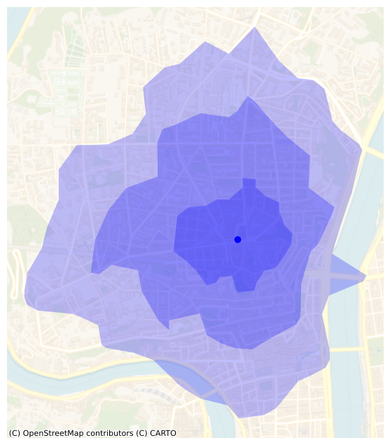
From the POI
5, 10 and 15 minutes “outward” isochrones.
isochrones_out = create_isochrones(
    coords, tt_col="tt_out", x_col="x_2154", y_col="y_2154", steps_m=steps
)
ax = isochrones_out.plot(alpha=0.25, color="b", figsize=FS)
cx.add_basemap(
    ax,
    source=xyz.CartoDB.VoyagerNoLabels,
    crs=isochrones_out.crs.to_string(),
    alpha=0.8,
)
_ = plt.plot(poi_lam93.x, poi_lam93.y, "bo")
_ = plt.axis("off")

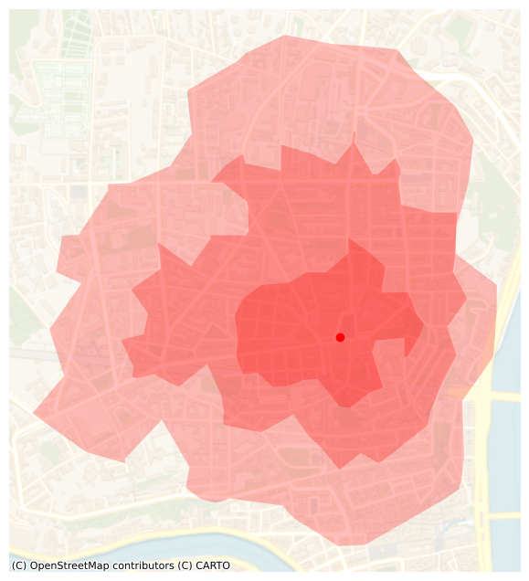
To the POI
5, 10 and 15 minutes “inward” isochrones.
isochrones_in = create_isochrones(
    coords,
    tt_col="tt_in",
    x_col="x_2154",
    y_col="y_2154",
    steps_m=steps,
)
ax = isochrones_in.plot(alpha=0.25, color="r", figsize=FS)
cx.add_basemap(
    ax,
    source=xyz.CartoDB.VoyagerNoLabels,
    crs=isochrones_out.crs.to_string(),
    alpha=0.8,
)
_ = plt.plot(poi_lam93.x, poi_lam93.y, "ro")
_ = plt.axis("off")

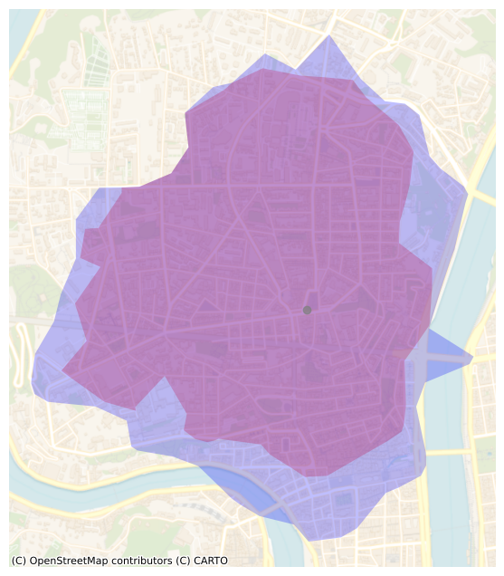
Overlap
We keep the same colors as before:
- from the POI in blue
- to the POI in red
t = 15  # 15 minutes
ax = isochrones_in.loc[[t]].plot(alpha=0.25, color="r", figsize=FS,label="in")
ax = isochrones_out.loc[[t]].plot(alpha=0.25, color="b",  ax=ax, label="out")
cx.add_basemap(
    ax, source=cx.providers.CartoDB.VoyagerNoLabels, crs=isochrones_out.crs.to_string()
)

_ = plt.plot(poi_lam93.x, poi_lam93.y, marker="o", color="grey", alpha=0.7)
_ = plt.axis("off")

The plot reveals a small discrepancy between the area that can be reached within 15 minutes from the hilltop and the area that can be reached within 15 minutes to the hilltop. As someone who lives near this POI, I can confirm that the difference between the “from” and “to” 15-minutes isochrones is quite significant. I guess that I tend to walk faster downhill and slower uphill than what is predicted by Tobler’s hiking function.