Enrich a digital terrain model
In this blog post, we will explore how to enrich a digital terrain model (DTM) using Python. We are going to use a DTM raster file of the region of Lyon, France, which was created in a previous post using data from the French National Geographic Institute (IGN): Lyon’s Digital Terrain Model with IGN Data. We will crop the DTM to a specific bounding box and enrich it with additional data using the efficient RichDEM package. Specifically, we will add slope and aspect data to the DTM, which can be used to analyze the steepness and orientation of the terrain.
Once we have enriched the DTM, we will save it to a new file and query it to extract data at specific locations. Finally, we will visualize hill shades with different azimuth and altitude angles.
Imports
import os

import contextily as cx
import earthpy.plot as ep
import earthpy.spatial as es
import geopandas as gpd
import matplotlib.pyplot as plt
import numpy as np
import pandas as pd
import rasterio as rio
import richdem as rd
from rasterio.mask import mask
from shapely.geometry import Polygon

FIGSIZE = (12, 8)

INPUT_DTM_FP = "./lyon_dtm.tif"  # input Digital Terrain Model (DTM) file path
CROPPED_DTM_FP = "./lyon_dem_cropped.tif"  # cropped DTM file path
OUTPUT_DTM_FP = "./lyon_dem_enriched.tif"  # enriched output DTM file path
System and package versions
We are operating on Python version 3.11.8 and running on a Linux x86_64 machine.
contextily : 1.6.0
earthpy    : 0.9.4
geopandas  : 0.14.3
matplotlib : 3.8.3
numpy      : 1.26.4
rasterio   : 1.3.9
richdem    : 2.3.0
shapely    : 2.0.3
First we need to load the data and crop the raster file with a bounding box expressed in the same Coordinate Reference System (CRS).
Crop the raster file to have an horizontal rectangle in EPSG:2154
Bounding box definition with longitude and latitude
We define the bounding box coordinates in EPSG:4326 (WGS 84) and create a polygon from the points.
# Define bounding box coordinates in EPSG:4326
bbox = (4.393158, 45.487095, 5.262451, 46.004593)
# Define points to create a polygon
point1 = (bbox[0], bbox[1])
point2 = (bbox[0], bbox[3])
point3 = (bbox[2], bbox[3])
point4 = (bbox[2], bbox[1])
# Create a polygon from the points
polygon_4326 = Polygon([point1, point2, point3, point4])
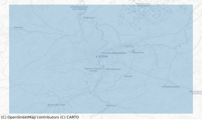
# display the polygon with map tiles
bbox_gs = gpd.GeoSeries([polygon_4326], crs="EPSG:4326")
fig, ax = plt.subplots(1, figsize=(8, 8))
ax = bbox_gs.plot(alpha=0.3, ax=ax)
cx.add_basemap(ax, crs=bbox_gs.crs.to_string(), source=cx.providers.CartoDB.Positron)
ax.set_axis_off()
CRS change to a projected CRS
Now we change the CRS of the bounding box to a projected CRS in order to match the CRS of the raster file. A projected CRS is a coordinate system that uses a flat, two-dimensional surface to represent the three-dimensional surface of the Earth. This is in contrast to a geographic CRS, which uses angles (latitude and longitude) to represent locations on the Earth’s surface. The raster file we are working with in this blog post uses a projected CRS (EPSG:2154 - Lambert 93), which is a common CRS for maps of France.
The geometry.values[0] part of the code is used to display the geometry in its new CRS.
# change the CRS
bbox_gs = bbox_gdf.to_crs("EPSG:2154")
bbox_gs.geometry.values[0]

Horizontal rectangle cropping
When we changed the CRS of the bounding box, the shape of the bounding box became distorted, and it is no longer an horizontal rectangle. In order to crop the raster file to a horizontal rectangle, we need to define a new bounding box that is an horizontal rectangle in the projected CRS. To do this, we extract the x and y coordinates of the previous bounding box using the exterior.xy attribute of the Shapely geometry object and try to find the largest horizontal rectangle contained in this quadrilateral.
We then create a new Shapely Polygon object from these four corner points. This new polygon represents the horizontal rectangle that we will use to crop the raster file.
xx, yy = bbox_gs.geometry.values[0].exterior.xy
xx = np.sort(np.unique(xx))
x_min, x_max = xx[1], xx[-2]
yy = np.sort(np.unique(yy))
y_min, y_max = yy[1], yy[-2]
bbox = (x_min, y_min, x_max, y_max)

# Define points to create a polygon
point1 = (bbox[0], bbox[1])
point2 = (bbox[0], bbox[3])
point3 = (bbox[2], bbox[3])
point4 = (bbox[2], bbox[1])

# Create a polygon from the points
polygon_lam93 = Polygon([point1, point2, point3, point4])
polygon_lam93

Load, crop and saved the cropped raster
The mask() function from rasterio is used to crop the input raster to the specified polygon, resulting in a cropped raster that covers only the area of interest.
input_raster = rio.open(INPUT_DTM_FP)

# Crop the raster to the bounding box
out_image, out_transform = mask(input_raster, [polygon_lam93], crop=True, filled=False)

out_meta = input_raster.meta
out_meta.update(
    {
        "driver": "GTiff",
        "height": out_image.shape[1],
        "width": out_image.shape[2],
        "transform": out_transform,
    }
)
# Save the cropped raster to a new GeoTIFF file
with rio.open(CROPPED_DTM_FP, "w", **out_meta) as dest:
    dest.write(out_image)
Enrich with RichDEM
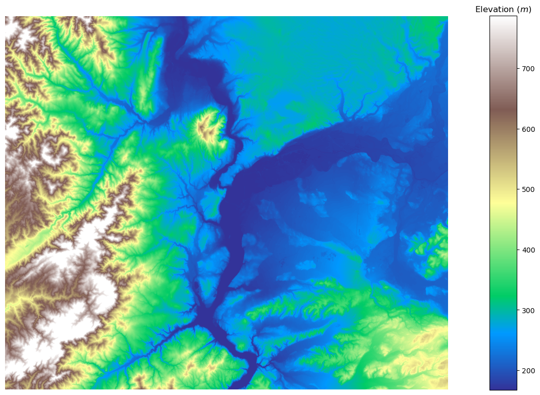
In this section, we start by loading the cropped DTM into RichDEM using the rd.LoadGDAL() function. We then use the rd.TerrainAttribute() function to calculate the slope and aspect of the terrain. Slope is a measure of the steepness of the terrain, while aspect is a measure of the direction that the slope is facing.
%%time
elevation = rd.LoadGDAL(CROPPED_DTM_FP)
CPU times: user 28.4 ms, sys: 247 ms, total: 275 ms
Wall time: 275 ms
_ = rd.rdShow(elevation, axes=False, cmap="terrain", show=False, figsize=FIGSIZE)
fig = plt.gcf()
ax = fig.gca()
_ = ax.set_title("Elevation ($m$)")
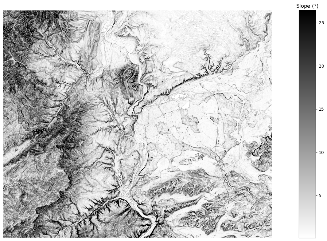
Slope
The slope calculation is performed using the method described by Berthold K.P. Horn [1], which calculates the slope in degrees based on the change in elevation between neighboring cells.
%%time
slope = rd.TerrainAttribute(elevation, attrib="slope_degrees")
CPU times: user 2.39 s, sys: 99.5 ms, total: 2.49 s
Wall time: 2.46 s
A Slope calculation (degrees)[39m
C Horn, B.K.P., 1981. Hill shading and the reflectance map. Proceedings of the IEEE 69, 14–47. doi:10.1109/PROC.1981.11918[39m
[2Kt Wall-time = 2.34489[39m ] (12% - 17.0s - 1 threads) ] (26% - 5.6s - 1 threads)
_ = rd.rdShow(slope, axes=False, cmap="binary", show=False, figsize=FIGSIZE)
fig = plt.gcf()
ax = fig.gca()
_ = ax.set_title("Slope ($°$)")
Aspect
The aspect calculation is also based on the method described by Berthold K.P. Horn [1], which calculates the aspect as the direction of the maximum rate of change of elevation.
%%time
aspect = rd.TerrainAttribute(elevation, attrib="aspect")
CPU times: user 4.35 s, sys: 122 ms, total: 4.47 s
Wall time: 4.39 s
A Aspect attribute calculation[39m
C Horn, B.K.P., 1981. Hill shading and the reflectance map. Proceedings of the IEEE 69, 14–47. doi:10.1109/PROC.1981.11918[39m
[2Kt Wall-time = 4.27062[39m ] (12% - 31.0s - 1 threads)
_ = rd.rdShow(
    aspect, axes=False, cmap="hsv", show=False, figsize=FIGSIZE
)  # cyclic colormap
fig = plt.gcf()
ax = fig.gca()
_ = ax.set_title("Aspect ($°$)")
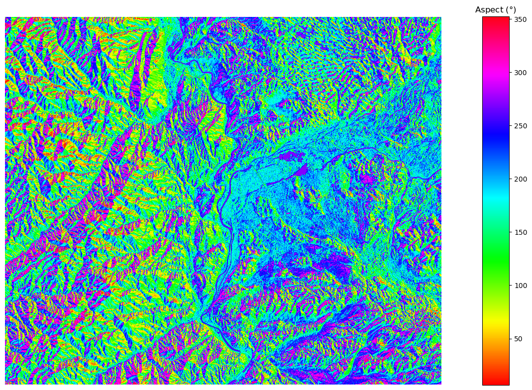
In the aspect plot, the azimuth angle represents the direction of the slope. The aspect values are typically represented in degrees clockwise from north (0°):
- 0°-360°: North. This means that the slope is facing towards the north. In other words, if you were to stand on the slope and face downhill, you would be facing north. Since 0° and 360° are equivalent, both values represent north.
- 90°: East.
- 180°: South.
- 270°: West.
In the aspect plot, the colors represent the different azimuth angles.
Note that we could also compute some curvature data with the RichDEM package.
Save the enriched DTM
In the following we save the enriched DTM by writing the elevation, slope, and aspect bands to a new GeoTIFF file using the rasterio library.
# Read metadata of first file
dtm = rio.open(CROPPED_DTM_FP)
meta = dtm.meta

bands = [elevation, slope, aspect]

# Update meta to reflect the number of layers
meta.update(count=len(bands))

# Read each layer and write it to stack
with rio.open(OUTPUT_DTM_FP, "w", **meta) as dst:
    for id, layer in enumerate(bands, start=1):
        dst.write_band(id, layer)
Query the enriched DTM
Here we use random coordinates, generated within the bounding box of the enriched DTM in order to show a query example. We query elevation, slope, and aspect values at those points using the sample() method from the rasterio library. The resulting data is stored in a pandas DataFrame.
rng = np.random.default_rng(421)

# Set the number of random coordinates you want
num_points = 1000

# Generate random x, y coordinates within the bounding box
random_x = rng.uniform(dtm.bounds.left, dtm.bounds.right, num_points)
random_y = rng.uniform(dtm.bounds.bottom, dtm.bounds.top, num_points)
point_coords = list(zip(random_x, random_y))

point_df = pd.DataFrame(data={"x_2154": random_x, "y_2154": random_y})
%%time
dtm = rio.open(OUTPUT_DTM_FP)
point_df[["elevation", "slope", "aspect"]] = [x for x in dtm.sample(point_coords)]
CPU times: user 36.6 ms, sys: 23.6 ms, total: 60.1 ms
Wall time: 59.9 ms
point_df
| x_2154 | y_2154 | elevation | slope | aspect | |
|---|---|---|---|---|---|
| 0 | 820891.261579 | 6.538451e+06 | 383.420013 | 4.896277 | 309.077728 |
| 1 | 822310.025385 | 6.512176e+06 | 794.710022 | 23.744192 | 39.280010 |
| ... | ... | ... | ... | ... | ... |
| 998 | 839788.130515 | 6.539853e+06 | 226.509995 | 4.520816 | 321.934448 |
| 999 | 839614.164818 | 6.499597e+06 | 158.139999 | 0.551047 | 117.900581 |
1000 rows × 5 columns
Hill shade visualization
In the final section of this blog post, we will explore how to create hillshade visualizations of the enriched DTM using the hillshade() function from the earthpy.spatial module. Hillshading is a technique used to create a shaded relief map that gives the illusion of three-dimensional depth to a two-dimensional surface. I discoved this module thanks to a post from Nicolas Mondon, a data journalist who creates some great content.
The hillshade() function takes three arguments: the elevation raster, the azimuth angle, and the altitude angle.
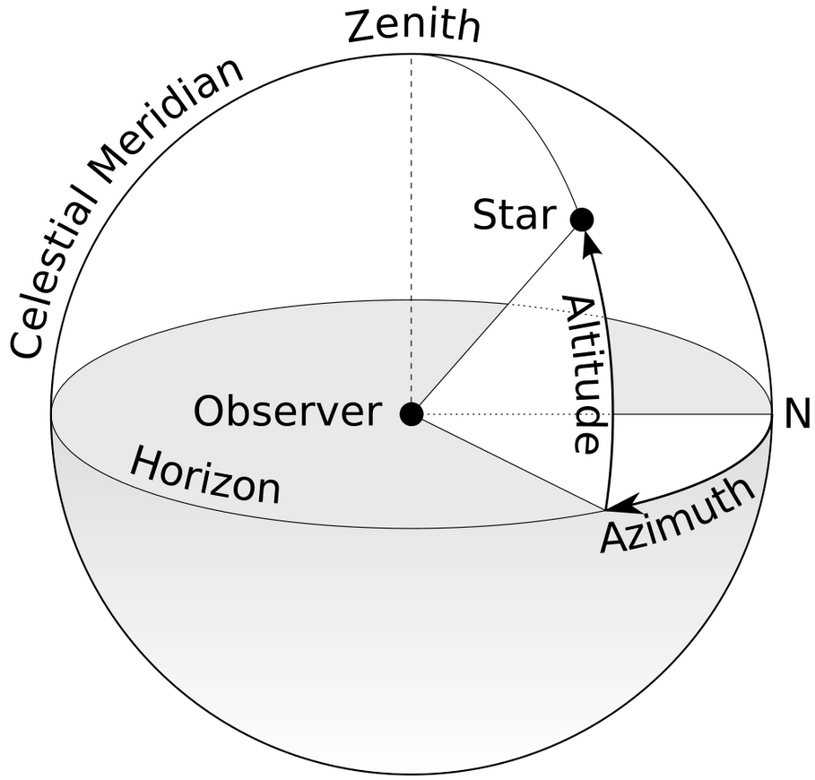
Source : wikipedia CC BY-SA 3.0
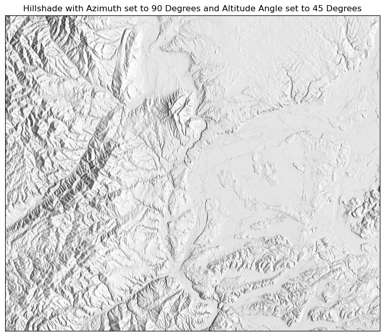
In the first example, we set the azimuth angle to 90 degrees and the altitude angle to 45 degrees.
azimuth = 90
altitude = 45

hillshade = es.hillshade(elevation, azimuth=azimuth, altitude=altitude)

# Plot the hillshade layer with the specified azimuth and altitude
_ = ep.plot_bands(
    hillshade,
    cbar=False,
    title=f"Hillshade with Azimuth set to {azimuth} Degrees and Altitude Angle set to {altitude} Degrees",
    figsize=FIGSIZE,
)
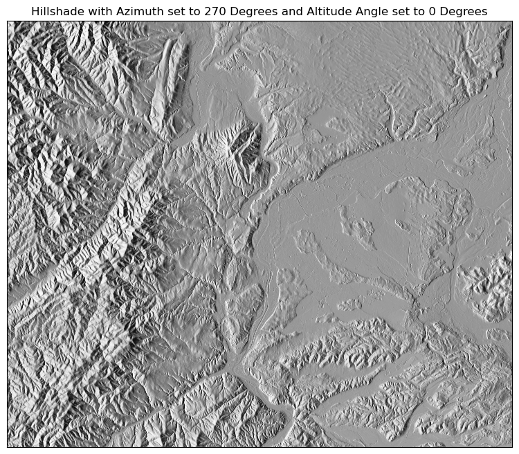
In the second example, we set the azimuth angle to 270 degrees and the altitude angle to 0 degrees.
azimuth = 270
altitude = 0

hillshade = es.hillshade(elevation, azimuth=azimuth, altitude=altitude)

# Plot the hillshade layer with the specified azimuth and altitude
_ = ep.plot_bands(
    hillshade,
    cbar=False,
    title=f"Hillshade with Azimuth set to {azimuth} Degrees and Altitude Angle set to {altitude} Degrees",
    figsize=FIGSIZE,
)
Reference
[1] Horn, B. K. P., “Hill shading and the reflectance map”, IEEE Proceedings, vol. 69, IEEE, pp. 14–47, 1981.