Dijkstra’s algorithm in Cython, part 1/3

In this post, we are going to present an implementation of Dijkstra’s algorithm in Cython. Dijkstra’s algorithm is a shortest path algorithm. It was conceived by Edsger W. Dijkstra in 1956, and published in 1959 [1].

Credit: Wikimedia Commons (CC BY-SA 3.0)

From a directed graph $\mathcal{G}=(V, E)$ with non-negative edge weights $w$, we want to compute the shortest weighted path from a source vertex to all graph vertices. This is why we refer to this algorithm as Single Source Shortest Path (SSSP). A path is a sequence of edges which joins a sequence of vertices. The cost or weight of a path is the sum of the weights of its constituent edges.

There are many variants and evolutions of this algorithm but we focus here on this classical one-to-all version. In the present implementation, we are not going to store the shortest paths, but only the cost associated with the shortest path at each vertex. However, Dijkstra’s algorithm can be built using an array of predecessors: for each vertex $v$, we would store the previous vertex index in the shortest path from the source vertex $s$ to $v$. Then, it is easy to trace backward the shortest path from any destination vertex to the origin $s$.

The use cases here are road networks, with rather sparse networks. We are going to run the SSSP algorithm on the DIMACS road networks that we downloaded in a previous post: Download some benchmark road networks for Shortest Paths algorithms .

New York network

New York road network from the DIMACS implementation challenge

Also, we are going to use the min-prioriy queue, based on a binary heap, presented in another post: A Cython implementation of a priority queue. The heap elements correspond to graph vertices, with the key value being the travel time from the source.

SSSP algorithm

Here is a short description of the algorithm from Cormen et al. [2]:

Dijkstra’s algorithm maintain a set $S$ of vertices whose final shortest-path weights from the source $s$ have already been determined. The algorithm repeatedly selects the vertex $u \in V-S$ with the minimum shortest-path estimate, adds $u$ to $S$, and relaxes all edges leaving $u$.

A the beginning of the algorithm, all vertices $v$ but the source are initialized with an infinite key value. Relaxation is the process of decreasing this key value when a shorter path to this vertex $v$ has been found. Relaxation is done for a vertex when the shortest path weight has been reached.

However, there are two variants regarding the initialization of the heap. As described on the wikipedia page:

Instead of filling the priority queue with all nodes in the initialization phase, it is also possible to initialize it to contain only source.

We tested both versions. Let’s start with the simplest version where the queue is filled with all vertices.

First approach: initialize the priority queue with all nodes

The algorithm can be decomposed in the following steps:

initialization:
- $S=\emptyset$. $S$ is the set of “scanned” vertices for which the shortest path has been evaluated and won’t be modified anymore.
- insert all vertices $v$ but $s$ into the priority queue $Q$ with an infinite key value: $v.key=\infty$
- insert the source vertex $s$ into $Q$ with a 0 key value: $s.key=0$
loop:
- while $Q$ is not empty
  - extract the element $u$ from $Q$ with min priority
  - add $u$ to $S$
  - for each outgoing edge $(u, v) \in E$:
    - if $v \notin S$ and $v.key > u.key + w(u,v)$:
      - decrease key of $v$ with key value v_key $u.key + w(u,v)$

Second approach: initialize the priority queue with only the source

This time, only the source vertex $s$ is initially added to the queue:

initialization:
- $S=\emptyset$.
- insert the source vertex $s$ into $Q$ with a 0 key value: $s.key=0$
loop:
- while $Q$ is not empty
  - extract the element $u$ from $Q$ with min priority
  - add $u$ to $S$
  - for each outgoing edge $(u, v) \in E$:
    - if $v \notin S$:
      - if $v \notin Q$:
        
        insert $v$ into $Q$ with key value: $u.key + w(u,v)$
      - else:
        
        if $v.key > u.key + w(u,v)$:
        
        decrease key of $v$ with key value v_key $u.key + w(u,v)$

General idea

Without going into the details, the idea of this algorithm is quite simple: at each iteration, we consider the vertex $u$ with minimum key value of the queue, as a “candidate” to be added to the set $S$. This would means that a shortest path $p$, from $s$ to $u$, has been found.

But how can we be sure that there is not another distinct path $p’$ with a shorter cost? The source vertex $s$ is the first one to be added to $S$ at the first step of the loop. We know that the key value $s.key=0$ will not be updated ever. At the current iteration, the paths $p$ and $p’$ must go from $s$ inside of $S$ to the candidate vertex $u$, outside of $S$. At some point, both paths use an outgoing edge from a vertex inside of $S$ to a vertex outside of $S$. But all the head vertices of the edges leaving $S$ have previously been added to the queue in the algorithm. Because $u$ has a minimal key value in the queue, it implies that the path $p’$ has a cost at least equal to, but not smaller than, the cost of $p$.

In the following, we use an enum state for each vertex $v$, i.e., to describe if $v$ is in $S$, in $Q$, or neither:

SCANNED: $v \in S$
IN_HEAP: $v \in Q$
NOT_IN_HEAP: $v \notin S$ and $v \notin Q$

Cython implementation

The Cython implementation makes use of two important components presented in previous posts:

the Cython priority queue : A Cython implementation of a priority queue
the forward star representation of the graph, in NumPy arrays: Forward and reverse stars in Cython

The forward star representation is allowing an efficient access to the outgoing edges from a given node. We would use the reverse star to access the incoming edges, in the case of a Single Target Shortest Path algorithm, to compute the shortest paths from any node in the graph to a target node.

The Cython code for the priority queue (pq_bin_heap_basic) and the forward star representation have been placed into Cython modules. The code is taken straightly from the indicated posts. The following implementation corresponds to the second approach, in which only the source vertex is inserted in the queue at the beginning.

import numpy as np
cimport numpy as cnp

cimport pq_bin_heap_basic as bhb

DTYPE = np.float64
ctypedef cnp.float64_t DTYPE_t

cpdef cnp.ndarray path_length_from_bin_basic(
    cnp.uint32_t[::1] csr_indices,
    cnp.uint32_t[::1] csr_indptr,
    DTYPE_t[::1] csr_data,
    int origin_vert_in,
    int vertex_count):
    """ Compute single-source shortest path (one-to-all)
        using a priority queue based on a binary heap.
    """

    cdef:
        size_t tail_vert_idx, head_vert_idx, idx  # indices
        DTYPE_t tail_vert_val, head_vert_val  # vertex travel times
        bhb.PriorityQueue pqueue 
        bhb.ElementState vert_state  # vertex state
        size_t origin_vert = <size_t>origin_vert_in

    with nogil:

        # initialization of the heap elements 
        # all nodes have INFINITY key and NOT_IN_HEAP state
        bhb.init_pqueue(&pqueue, <size_t>vertex_count)

        # the key is set to zero for the origin vertex,
        # which is inserted into the heap
        bhb.insert(&pqueue, origin_vert, 0.0)

        # main loop
        while pqueue.size > 0:
            tail_vert_idx = bhb.extract_min(&pqueue)
            tail_vert_val = pqueue.Elements[tail_vert_idx].key

            # loop on outgoing edges
            for idx in range(<size_t>csr_indptr[tail_vert_idx], <size_t>csr_indptr[tail_vert_idx + 1]):
                head_vert_idx = <size_t>csr_indices[idx]
                vert_state = pqueue.Elements[head_vert_idx].state
                if vert_state != bhb.SCANNED:
                    head_vert_val = tail_vert_val + csr_data[idx]
                    if vert_state == bhb.NOT_IN_HEAP:
                        bhb.insert(&pqueue, head_vert_idx, head_vert_val)
                    elif pqueue.Elements[head_vert_idx].key > head_vert_val:
                        bhb.decrease_key(&pqueue, head_vert_idx, head_vert_val)

    # copy the results into a numpy array
    path_lengths = cnp.ndarray(vertex_count, dtype=DTYPE)

    cdef:
        DTYPE_t[::1] path_lengths_view = path_lengths

    with nogil:

        for i in range(<size_t>vertex_count):
            path_lengths_view[i] = pqueue.Elements[i].key

    # cleanup
    bhb.free_pqueue(&pqueue)  

    return path_lengths

Because we do not want the post to be loaded with too many lines of code, we do not show here the Python code to load the graphs into dataframes, convert them into the forward star representation (csr_indices, csr_indptr and csr_data). For the same reason, we do now show the implementation of the first approach neither (initialize the priority queue with all nodes).

A Visualization of the algorithm

The following animated gif has been made in two steps. Some printf statements have been added to the above code to print the vertex indices (added to and removed from the heap) at each step of the iteration. Then using this “trace” text file and the vertex coordinates, some figures have been generated every 1000 steps. Vertices in the heap are colored in red while those that have been scanned are in blue. We can observe the front propagation process of the algorithm.

Dijkstra

Animation of Dijkstra's algorithm (second approach) applied to the New York road network

This New York network has 3730100 edges and 264346 vertices. It is interesting to observe that in this second approach, the heap size remains relatively small compared to the number of vertices.

heap size NY

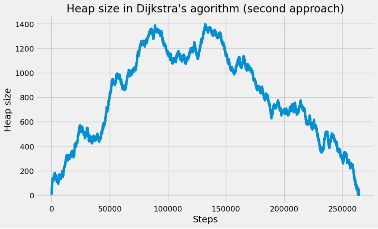
The heap size figure and the animated gif corresponds to the same run (New York network), with source node index idx_from = 1000.

Validation and infinite travel time

Results from our path_length functions have been checked against SciPy (scipy.sparse.csgraph.dijkstra):

path_lengths_ref = dijkstra(
    csgraph=graph_csr, directed=True, indices=idx_from, return_predecessors=False
)

When a node cannot be reached from the source vertex $s$, its key value remains the initial infinite value. Because we do not deal with infinity in the Cython code, we use the largest value of the DTYPE data type, i.e.:

DTYPE_INF_PY = np.finfo(dtype=np.float64).max

However, the SciPy dijkstra function returns np.inf values for these nodes, so we need do replace these DTYPE_INF_PY values with np.inf ones in order to get the same output:

# deal with infinity
path_lengths = np.where(
    path_lengths == DTYPE_INF_PY, np.inf, path_lengths
)

Then we can compare the different results with the following command:

assert np.allclose(
    path_lengths, path_lengths_ref, rtol=1e-05, atol=1e-08, equal_nan=True
)

Execution timings

Let’s compare the two approaches on the USA network, 57708624 edges and 23947347 vertices. These algoritms have two distinct phases: setup and run. During the setup phase, the graph data structured are prepared for the algorithm to run. This setup phase only needs to be run once for any number of calls to the path_length functions. In the following, we only measure the execution time of the run phase. We use the best time over 3 runs.

heap init strategy

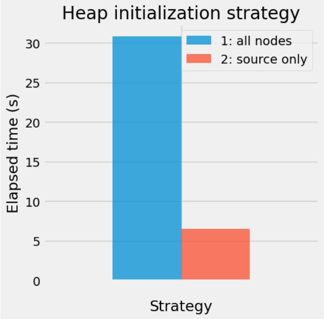
We can see that the second strategy is far more efficient. This may be due to the fact that the heap size remains smaller in the second approach, and that the decrease_key operation is expensive as compared to the insert one.

In the following posts, we will study various priority queue versions, and compare the resulting implementation with some shortest path libraries available in Python.

References

[1] Dijkstra, E. W., A note on two problems in connexion with graphs, Numerische Mathematik. 1: 269–271 (1959), doi:10.1007/BF01386390.

[2] Cormen et al., Introduction to Algorithms, MIT Press and McGraw-Hill, coll. « third », 2009.