Dijkstra's algorithm in Cython, part 3/3
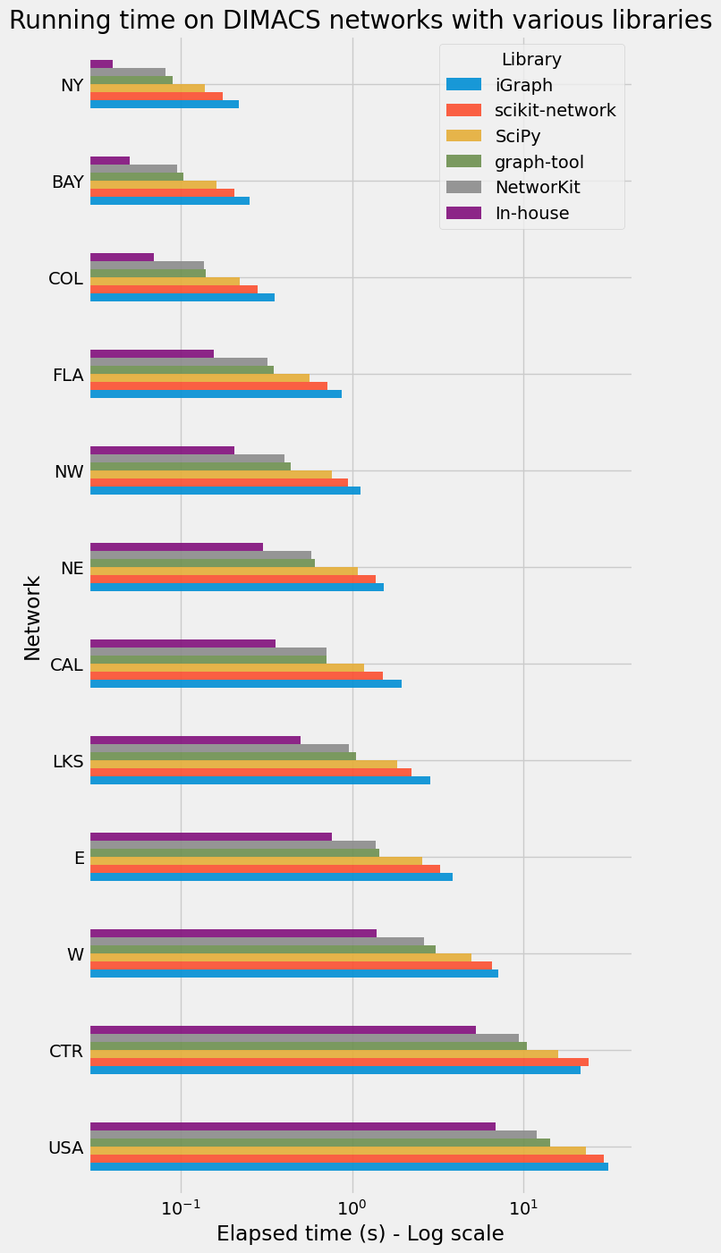
Running time of Dijkstra’s algorithm on DIMACS networks with various implementations in Python.
This post is the last part of a three-part series:
In the present post, we compare the in-house implementation of Dijkstra’s algorithm described in the previous posts with other implementations available in Python. Here are the shortest path libraries that we used:
- iGraph: Python interface of igraph, a fast and open source C library to manipulate and analyze graphs
- scikit-network: Python package for the analysis of large graphs
- SciPy: fundamental algorithms for scientific computing in Python
- graph-tool: efficient Python module for manipulation and statistical analysis of graphs
- NetworKit: NetworKit is a growing open-source toolkit for large-scale network analysis
We apply the shortest path routines to the DIMACS road networks, downloaded in a previous post: Download some benchmark road networks for Shortest Paths algorithms . Here is a summary of the DIMACS networks features:
| name | vertex count | edge count | mean degree |
|---|---|---|---|
| NY | 264346 | 730100 | 2.76 |
| BAY | 321270 | 794830 | 2.47 |
| COL | 435666 | 1042400 | 2.39 |
| FLA | 1070376 | 2687902 | 2.51 |
| NW | 1207945 | 2820774 | 2.34 |
| NE | 1524453 | 3868020 | 2.54 |
| CAL | 1890815 | 4630444 | 2.45 |
| LKS | 2758119 | 6794808 | 2.46 |
| E | 3598623 | 8708058 | 2.42 |
| W | 6262104 | 15119284 | 2.41 |
| CTR | 14081816 | 33866826 | 2.41 |
| USA | 23947347 | 57708624 | 2.41 |
Similarly to what we did in the previous post, we call Dijkstra’s algorithm to get the shortest distance from one node (idx_from = 1000) to all other nodes. We do not store the shortest path, or predecessors, but only the vertex distance from source vertex. Although we call it distance, this corresponds to the shortest path weight, whatever does the edge weight represent.
Code samples
In the following you will find some code snippets describing how we called each library. However, for the sake of brevity, we did not include all the code used to measure the running time in this post.
Package versions
Here are the versions of the packages used to run Dijkstra’s algorithm.
Python version       : 3.10.8
igraph               : 0.10.2
sknetwork            : 0.28.2
scipy                : 1.9.3
graph_tool           : 2.45
networkit            : 10.0
cython               : 0.29.32
numpy                : 1.23.5
Load the networks
At first, we need to load the network, as a Pandas dataframe in COO format, and as NumPy arrays in CSR format (forward star representation):
import pandas as pd
from scipy.sparse import coo_array

# load into a dataframe
edges_df = pd.read_parquet(network_file_path)
edges_df.rename(
    columns={"id_from": "source", "id_to": "target", "tt": "weight"}, inplace=True
)
vertex_count = edges_df[["source", "target"]].max().max() + 1

# convert to CSR format
data = edges_df["weight"].values
row = edges_df["source"].values
col = edges_df["target"].values
graph_coo = coo_array((data, (row, col)), shape=(vertex_count, vertex_count))
graph_csr = graph_coo.tocsr()
Now we show small examples of calls to each of the external shortest path libraries, with a setup phase, if required, and a run phase.
iGraph
from igraph import Graph

# setup
# -----
g = Graph.DataFrame(edges_df, directed=True)

# run
# ---
distances = g.distances(
    source=idx_from, target=None, weights="weight", mode="out"
)
dist_matrix = np.asarray(distances[0])
scikit-network
from sknetwork.path import get_distances

# run
# ---
dist_matrix = get_distances(
    adjacency=graph_csr,
    sources=idx_from,
    method="D",
    return_predecessors=False,
    unweighted=False,
    n_jobs=1,
)
SciPy
from scipy.sparse.csgraph import dijkstra

# run
# ---
dist_matrix = dijkstra(
    csgraph=graph_csr,
    directed=True,
    indices=idx_from,
    return_predecessors=False,
)
graph-tool
import graph_tool as gt

# setup
# -----
g = gt.Graph(directed=True)
g.add_vertex(vertex_count)
g.add_edge_list(edges_df[["source", "target"]].values)
eprop_t = g.new_edge_property("float")
g.edge_properties["t"] = eprop_t  # internal property
g.edge_properties["t"].a = edges_df["weight"].values

# run
# ---
dist = topology.shortest_distance(
    g,
    source=g.vertex(idx_from),
    weights=g.ep.t,
    negative_weights=False,
    directed=True,
)
dist_matrix = dist.a
NetworKit
import networkit as nk

# setup
# -----
g = nk.Graph(n=vertex_count, weighted=True, directed=True, edgesIndexed=False)
for row in edges_df.itertuples():
    g.addEdge(row.source, row.target, w=row.weight)
nk_dijkstra = nk.distance.Dijkstra(
    g, idx_from, storePaths=False, storeNodesSortedByDistance=False
)

# run
# ---
nk_dijkstra.run()
dist_matrix = nk_dijkstra.getDistances(asarray=True)
dist_matrix = np.asarray(dist_matrix)
dist_matrix = np.where(dist_matrix >= 1.79769313e308, np.inf, dist_matrix)
In-house implementation
The Cython code for the priority queue based on a 4-ary heap has been placed into a Cython module. This implementation was described in the part 2/3 post. It is also based on a forward star representation of the graph, as described in the post: https://aetperf.github.io/2022/11/04/Forward-and-reverse-stars-in-Cython.html.
Running time
First of all, we check the output distance vectors of each implementation against SciPy. We use a t3.2xlarge EC2 instance with Ubuntu Linux to perform all the time measures. This way we are sure that the Python process has a large priority and that the running time is stable. We take the best running time over 10 consecutive runs.
Similarly to the previous part of the post series, we only measure the execution time of the run phase (not the setup phase). This is important because the setup phase may be rather long, if it involves a Python loop for example. We did not try to optimize this setup phase, which is performed only once before the 10 runs.
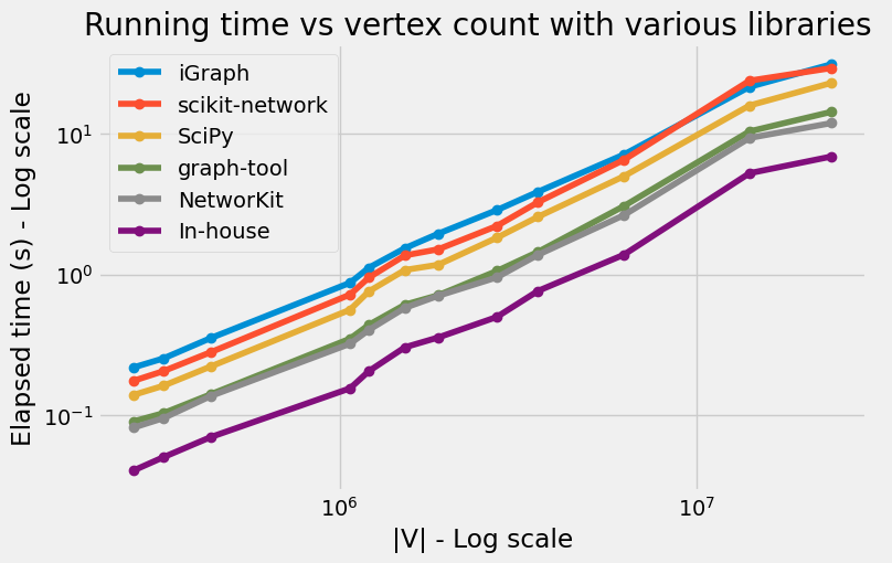
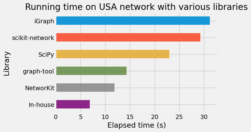
Results
Conclusion
We implemented Dijksta’s algorithm from scratch in Python using NumPy arrays and Cython. Cython is a really great tool, which makes writing efficient C extensions for Python as easy as Python itself.
This implementation is also based on 2 important data structures:
- the forward star representation of the graph
- the priority queue based on an implicit d-ary heap This combination leads to interesting results on the DIMACS road networks, actually faster than the great packages that we tried in this post.
There is still room for improvement. For example, we could try using a priority queue that does not support the decrease-key operation [1], or a monotone priority queue.
Reference
[1] Chen, M., Measuring and Improving the Performance of Cache-efficient Priority Queues in Dijkstra’s Algorithm, 2007.